| Characteristic | Beta1 | SE | 95% CI | p-value |
|---|---|---|---|---|
| (Intercept) | -0.01 | 0.017 | -0.04, 0.03 | 0.7 |
| vehicles | 0.02** | 0.008 | 0.01, 0.04 | 0.002 |
| hhsize | -0.03*** | 0.007 | -0.04, -0.01 | <0.001 |
| factor(income) | ||||
| 0 | — | — | — | |
| 35000 | 0.02 | 0.014 | -0.01, 0.04 | 0.2 |
| 75000 | 0.06** | 0.020 | 0.02, 0.10 | 0.002 |
| 100000 | 0.05** | 0.018 | 0.02, 0.09 | 0.005 |
| HTRESDN | 0.00 | 0.000 | 0.00, 0.00 | >0.9 |
| workers | 0.35*** | 0.008 | 0.33, 0.36 | <0.001 |
| R² | 0.280 | |||
| Adjusted R² | 0.279 | |||
| Statistic | 470 | |||
| p-value | <0.001 | |||
| No. Obs. | 8,476 | |||
| Residual df | 8,468 | |||
| Abbreviations: CI = Confidence Interval, SE = Standard Error | ||||
| 1 *p<0.05; **p<0.01; ***p<0.001 | ||||
Transportation modeling and engineering
Matt Bhagat-Conway
What is a travel demand model?
- A mathematical model (think regression, but more complicated) that simulates how much travel will occur with different demographic and transport network scenarios
Why model transportation?
- Transportation is a big investment
- Government spending on transport was ~1.2% of US GDP in 2016
- Interstate highways cost $2 million–$20+ million per lane-mile to build
- The Second Avenue Subway in New York City cost $2.5 billion per mile
- Though this is much higher than comparable projects
- The Texas Transportation Institute estimates congestion costs the US economy $100 billion per year
- Though this supposes the alternative of no congestion is possible
Why model transportation? Long-term
- Transportation is a long-term investment
- The bones of the interstate highway system were laid out in the 1950’s
- The East End Connector in Durham was first proposed in the 1950’s, formally planned in the 1980’s, and opened in 2022
- The WMATA (Washington, DC) Silver Line extension to Dulles International Airport was planned in the 1960’s when the airport opened and just finished in 2022
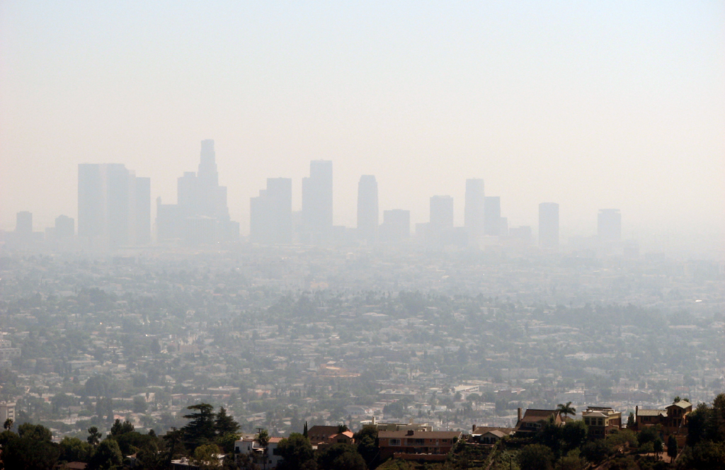
Why model transportation? Emissions
- The EPA defines six “criteria air pollutants” that are used to determine if an area is in compliance with federal air quality standards
- Ozone, particulate matter (\(\mathrm{PM}_{2.5}\) and \(\mathrm{PM}_{10}\)), lead, carbon monoxide, sulfur dioxide, nitrogen dioxide
- Many of these come from transportation, and modeling future transportation plans helps plan to keep these within EPA limits
- In air quality non-attainment areas, additional modeling requirements apply
The transportation modeling process
- All metropolitan planning organizations (MPOs) must produce a long range transportation plan (at least 20 years, but often 30-40)
- The current CAMPO plan for the Triangle forecasts to 2055
- These plans include proposed changes to the transportation network and forecasted demographics and land use
- They forecast several key outcomes: vehicle miles traveled (VMT), congestion levels, mode splits (i.e. car/transit/walk/bike/other), and emissions
The workhorse of travel demand modeling: the four-step model
- Pretty much every metropolitan planning organization (MPO) or state department of transportation has a travel demand model
- Many if not most of these are some variation of the four-step model
- Originally developed in the 1950s, though many improvements have been made since
- In the homework, you’ll run a four-step model of your own
The four steps of the four-step model
- Trip generation
- Estimate how many trips will be produced by and attracted to each travel analysis zone (TAZ)
- Trip distribution
- Estimate how many of the trips produced by a zone will be attracted to each other zone
- Mode choice
- How many of the trips between each pair of zones will be made by car, transit, bike, walk, etc.
- Agencies in heavily car-oriented areas may skip this step
- Network assignment/route choice
- What roads do the trips from A to B take?
- What does this mean for congestion levels?
Data sources for travel forecasting: the household travel survey
- The most important dataset for model development is a household travel survey
- Most regions conduct one every few years
- Households report their demographics and complete a travel diary—a list of all the trips they made during an assigned period (usually a day, but some agencies do multi-day surveys)
- GPS and smartphones have significantly reduced the respondent burden for travel diaries
Trip generation: the basics
- We need to know how many trips are produced in and attracted to each zone
- We are not forecasting at this point how many trips go from A to B, just:
- how many trips leave A going anywhere (production)
- how many trips go to B from anywhere (attraction)
Trip generation: types of trips
- Travel demand models classify trips into (at least) three types
- Home-based work: trips between home and work (in either direction)
- Home-based other: trips between home and non-work locations (in either direction)
- Non-home-based: trips between non-home locations
- Many models will further divide into home-based shopping, school trips, school dropoff on work tours, etc.
- A tour is a set of trips starting and ending at the same location
Trip generation methods: regression
- We develop a regression based on our travel survey to predict how many trips of a particular type a household will make
- We then apply this to all households in a zone, based on Census data or projections, to estimate how many trips will be produced in that zone
- Home-based trips are generally always considered to be produced at the home end, regardless of direction
Trip generation methods: regression example
This is the AM Peak home-based work regression from the model you’ll use in the homework.
Trip generation methods: cross-classification
- Another (probably more common) method for trip generation modeling is cross-classification
- Here, you create a table dividing households or land uses by common characteristics, and just compute the mean trips for each type of trip and household/land use
- You then apply those rates to Census data or demographic forecasts to estimate the number of trips produced by each zone
Trip generation methods: trip attractions
- For the attractions (non-home ends of trips), we can’t use Census data or demographic forecasts, because those only tell use where people live
- Instead, we generally use employment counts (projected or from the US Census LODES dataset), or land uses
- If using employment, it’s good to use employment in several sectors, in addition to total employment
- e.g. retail or medical employment will attract more daily trips per job
Trip generation outputs


Trip generation: balancing
- We almost never have a matching number of productions and attractions, but of course this doesn’t reflect the real world
- We’re generally more confident in the quality of our estimations of trip productions, so we
fudgeadjust or balance the total attractions to match the total productions
Trip distribution
- After trip generation, we have forecasted how many trips are produced by the residents of each area, and how many trips end in each area, but we don’t know which productions match which attractions
- What variables might be important to figure this out?
Trip distribution theory
\[ \frac{m_1 m_2}{d^2} \]
- Anyone recognize this equation?
Trip distribution theory: conceptually
- We theorize that the number of trips between two locations is proportional to the sizes of the locations, and inversely proportional to the difficulty of travel between them
- This makes intuitive sense
- For example, consider airline flights
- There are about 70 flights a day from New York to Chicago (733 miles)
- There are only 12 flights a day from Raleigh-Durham to Chicago (646 miles)
- Because Raleigh-Durham is smaller than New York (~2 million people vs ~20 million)
- There is only one flight a day from São Paulo (~22 million people) to Chicago
- Because São Paulo is much further away, 5,222 miles
The gravity model
- One common method for trip distribution is the gravity model:
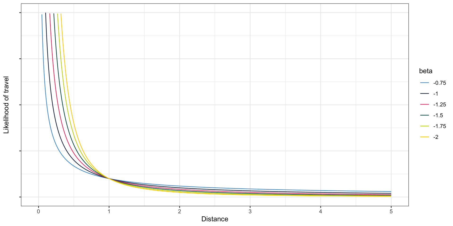
\[ t_{ij} \propto \frac{p_i a_j}{d_{ij}^\beta} \]
where \(t_{ij}\) is the number of trips from \(i\) to \(j\), \(p_i\) is the number of trips produced at \(i\), \(a_j\) is the number of trips attracted by \(j\), and \(d_{ij}\) the distance between \(i\) and \(j\). \(\propto\) means proportional to
\(d_{ij}^\beta\) is called the friction of distance; \(\beta\) is estimated based on data
The gravity model
You may also see the gravity model written like this; in this case \(\beta\) is negative but otherwise it’s equivalent
\[ t_{ij} \propto p_a a_j d_{ij}^{\beta} \]
The \(\beta\) parameter
Other models: negative exponential
- You may also see negative exponential models
- These have a very slightly different functional form than gravity models
\[ t_{ij} \propto p_i a_j e^{\beta d_{ij}} \]
- They are called negative exponential because \(\beta\) should be negative
- What would it mean if \(\beta\) were positive? 🤔
Other models: intervening opportunities
- The intervening opportunities model bases estimates not on distance, but on how much is closer
- Conceptually, this makes a lot of sense: you might drive ten miles to a grocery store if there weren’t any closer grocery stores
- But if you passed 15 grocery stores on the way, you’d be much less likely to travel that full ten miles
- Not used much, but probably should be used more
Generalized cost
- Distance might mean:
- Straight-line distance
- Network distance
- Travel time
- A generalized cost
- This could be anything, or multiple things; e.g. it might be a combination of travel time and tolls, or travel time plus extra penalties for changing buses, etc.
Trip distribution with a gravity model

Mode choice
- We have now forecasted how many trips will occur between each zone at each time period, but we don’t know what mode they will use
- That is the role of the third step, mode choice
- Some MPOs skip this step if they have very little use of alternative modes in their region
Mode choice models
- Mode choice usually uses a discrete choice model, also known as a random utility model
- Most commonly, a multinomial logit or the slightly more complex nested logit
- Also called multinomial logistic regression and nested logistic regression
- These are more advanced forms of regression where the dependent variable is categorical rather than continuous
The multinomial logit model
- The multinomial logit model expresses the value of each alternative as a utility
- The utility functions that determine this utility look like regular linear regression equations
- Whichever alternative has the highest utility is the one that will be chosen
- Each utility function has an error term, so which one is the highest is probabilistic not deterministic
The multinomial logit model: the math
A (very simple) mode choice model might look like:
\[\begin{align*} U_{car} &= & \beta_{t} x_{t} + && \epsilon \\ U_{transit} &= \alpha_{transit} + & \beta_{t} x_{t} +& \beta_{i,transit} x_{i} + & \epsilon \\ U_{bike} &= \alpha_{bike} + & \beta_{t} x_{t} +& \beta_{i,bike} x_{i} + & \epsilon \end{align*}\]
where \(U\) is utility of each mode, \(t\) is travel time and \(i\) is income.
Nerd moment: the \(\epsilon\) are Gumbel rather than Normal distributed, because it makes the math easier.
The multinomial logit model: probabilities
The probability of choosing any mode (in this case car) is:
\[ p_{car} = P(U_{car} > \mathrm{all~other}~U) = \frac{e^{U_{car}}}{e^{U_{car}} + e^{U_{bike}} + e^{U_{walk}} + e^{U_{transit}}} \]
(I’m not expecting you to remember this formula, I just want to walk through the math)
- What happens if \(U_{car}\) gets bigger (e.g. because car travel time goes down)?
- What happens if \(U_{transit}\) gets bigger (e.g. because income goes down)?
- What happens if all of the \(U\)’s go up the same amount? 😱
Interpreting a multinomial logit model: what you need to know as a planner
- You can read the utility functions just like linear regressions
- Anything that is associated with an increase in utility is associated with an increased likelihood of choosing that option, and a decreased likelihood of choosing the others
- Coefficients have standard errors, and you can do hypothesis tests and significance testing just like in linear regression
The mode choice step
- The mode choice step applies a mode choice model to predict the probability that trips between each pair of tracts use each mode
- We then multiply these probabilities by the number of trips we previously forecasted between the tracts, to get the estimated number of trips by mode
- For instance, suppose we predict that for trips between two tracts, the probabilities of choosing each mode are:
- Car: 0.9
- Transit: 0.07
- Bike: 0.02
- Walk: 0.01
- If we predicted 100 trips between these tracts, we now disaggregate that to:
- 90 predicted car trips
- 7 predicted transit trips
- 2 predicted bike trips
- 1 predicted walk trip
Network assignment/route choice
- The final step (phew!) is network assignment, aka route choice
- Often, the main outputs of interest are congestion and vehicle miles traveled (VMT)
- To calculate these, we need to know not only what the car trips were, but also what routes they took
- The network assignment step takes car trips between locations, and routes them on the network, accounting for the congestion caused by each trip
- Some agencies with significant transit ridership also do transit assignment
Network assignment/route choice: equilibrium
- The challenge with network assignment is that we want to find an equilibrium solution
- But each trip affects the travel time of all other trips
- If the travel time on the freeway gets bad enough, people will divert to other roads
- So the route each trip takes is a function of the routes all the other trips take
- You can see how figuring this out might be computationally challenging
Network assignment/route choice: assigment
- The most common assignment is a static traffic assignment, where the total flow over the course of an hour on each link is estimated, with no additional temporal detail
- The common Frank-Wolfe algorithm does this iteratively
- First, all trips are assigned to the shortest path as if there were no congestion
- Then, congestion is calculated, and all trips are re-routed based on that level of congestion
- Some percentage of the trips are assigned to take the new route, while other stay on the old routes
- You repeat the process until the answer stops changing
The Frank-Wolfe algorithm
The fundamental diagrams
- How do we know how traffic volumes translate to congestion?
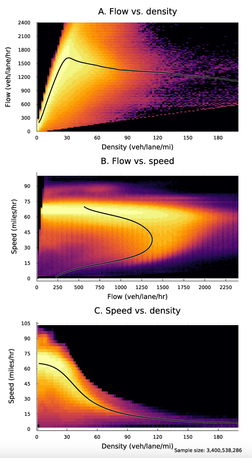
Bhagat-Conway and Zhang (2023)
The speed-flow diagram
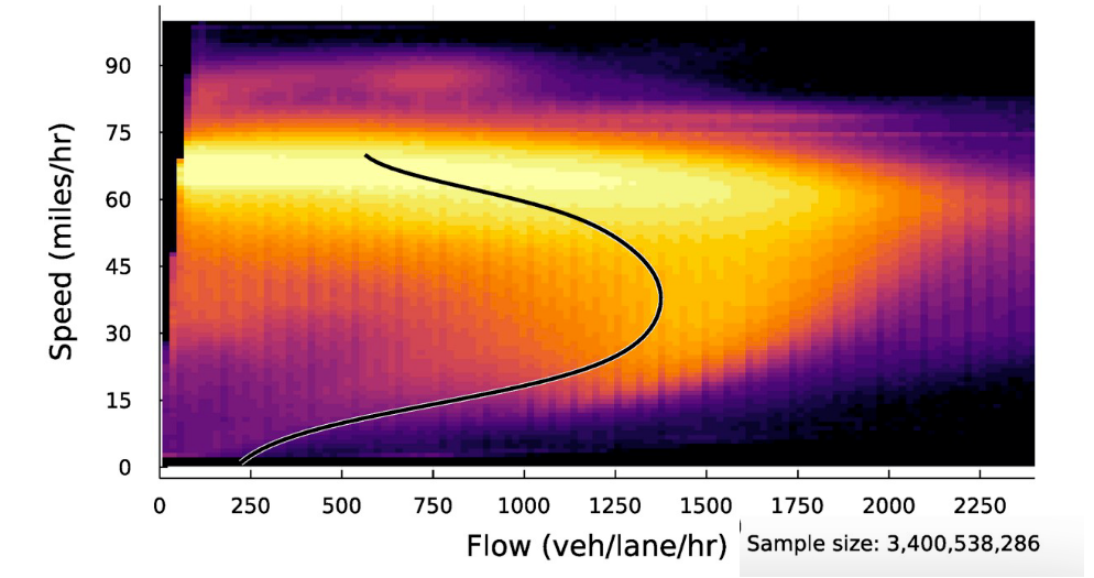
Bhagat-Conway and Zhang (2023)
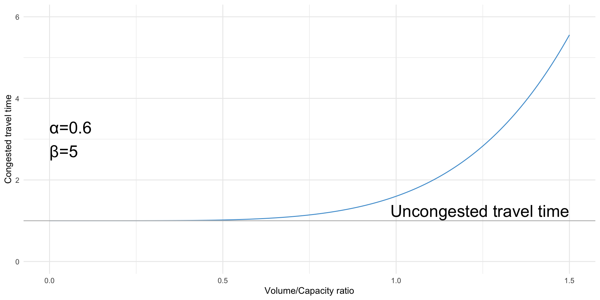
The Bureau of Public Roads function
The best-known formula for estimating congested travel time is the Bureau of Public Roads function, which estimates the congested travel time on a road segment as:
\[ tt_{congested} = tt_{uncongested} \cdot \left(1 + \alpha \left(\frac{v}{c}\right)^\beta \right) \]
where \(tt\) is travel time, \(v\) is the forecast volume on the segment, \(c\) is the capacity of the segment, and \(\alpha\) and \(\beta\) are parameters to estimate from data
The Bureau of Public Roads function
Additional components
- Emissions models
- External zones (traffic originating outside the region)
- Special generators/attractors: airports, universities, etc.
Criticisms of transportation modeling: land use is exogenous
- In most travel demand models, land use is treated as exogenous—i.e., taken as a given from projections or scenarios
- This means that you need to have a good land use forecast to get a good travel forecast
- Transportation affects land use just as land use affects transportation, so a really accurate model would model them jointly
- There is some progress on integrated land-use transportation models, but they are uncommon
Induced demand
- Induced demand is when you expand a road, and traffic eventually returns to what it was before
- This happens when additional demand is induced by the additional capacity: people switch from other modes, start commuting at rush hour instead of off-peak, or make trips they weren’t making before
- From an economic standpoint, when roads are free, congestion is the “cost” of using them
- When we lower the cost, more people will use the road
- Demand for roads is very elastic, so additional people will make trips until congestion (the “price”) is similar to what it was before
Induced demand and the four-step model
- Can the four-step model incorporate induced demand?
- Not the way we’ve set it up, anyways; sometimes some information about road capacity and congestion is added to distribution functions
- Sometimes models are iterated—run all the way through, and then information from the assignment is fed back into the distribution step to account for congestion
Criticisms of the four step model: does not match how people actually make decisions about travel
- The four-step model is pretty far removed from how people actually make decisions about travel
- No one goes “let’s see, I’ll make 2.3 trips today. Let’s see how many options are available for the other end of the trip, etc”
- The four-step model often works pretty well nonetheless, but it’s hard to test certain policies that might change behavior
Criticisms of modeling practice generally
- Many people criticize modeling as a predict and provide or self-fulfilling prohecy
- We model a future transportation network, build new highways based on the result, and then get the result we predicted, because we built it
The next generation of travel demand models: activity based models
- Four-step models are still the most common travel demand model used, especially in smaller cities
- But the new state of the art is the activity-based model
- Activity based models are disaggregate models: instead of modeling total flows, they individually simulate the decisions of all the households in the region
Activity based models
- They are computationally complex, but in many ways much more intuitive than four step models
- First, you generate a synthetic population: data on each household in the region
- Since we can’t actually collect this, we use Census data to create fake households that in aggregate resemble the actual population
- The core of the model is a set of dozens of regressions, modeling a slew of household- and person-level decisions
- e.g. destination choice, departure time choice, mode choice, etc.
- Each individual or “agent” gets their own schedule of where they’re going when
- These are aggregated to produce outputs
Activity-based model components
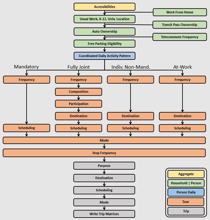
Components of ActivitySim
Transportation engineering
- Transportation engineering is distinct from transportation planning
- Generally, much more concerned with physical infrastructure and small-scale or short-term projects
- Planners can tell you where to build a bridge, but I wouldn’t recommend driving on a bridge built by a planner
Design guides: MUTCD, HCM, Green Book, Trip Generation Manual, NACTO guides
- Traffic engineering tends to be much more formulaic than planning
- There are a myriad of design guides that engineers use for different aspects of planning
- This can lead to clashes between engineers and planners
Roadway geometry
- The design and layout of roadways is heavily dependent on design guidance from a number of standards agencies
- AASHTO
- NACTO
- Deviating from these guidelines is often difficult, and a major source of friction between planners and engineers
Design vehicles, control vehicles, and managed vehicles
- One of the key inputs to the geometric design of roadways is the selection of the design vehicle
- This is the largest vehicle regularly expected to use the roadway, from a standardized list of vehicles in the AASHTO green book
- The selection of this vehicle has a very significant effect on the design of the roadway, including lane widths but especially turn radii
Design vehicles and turning templates
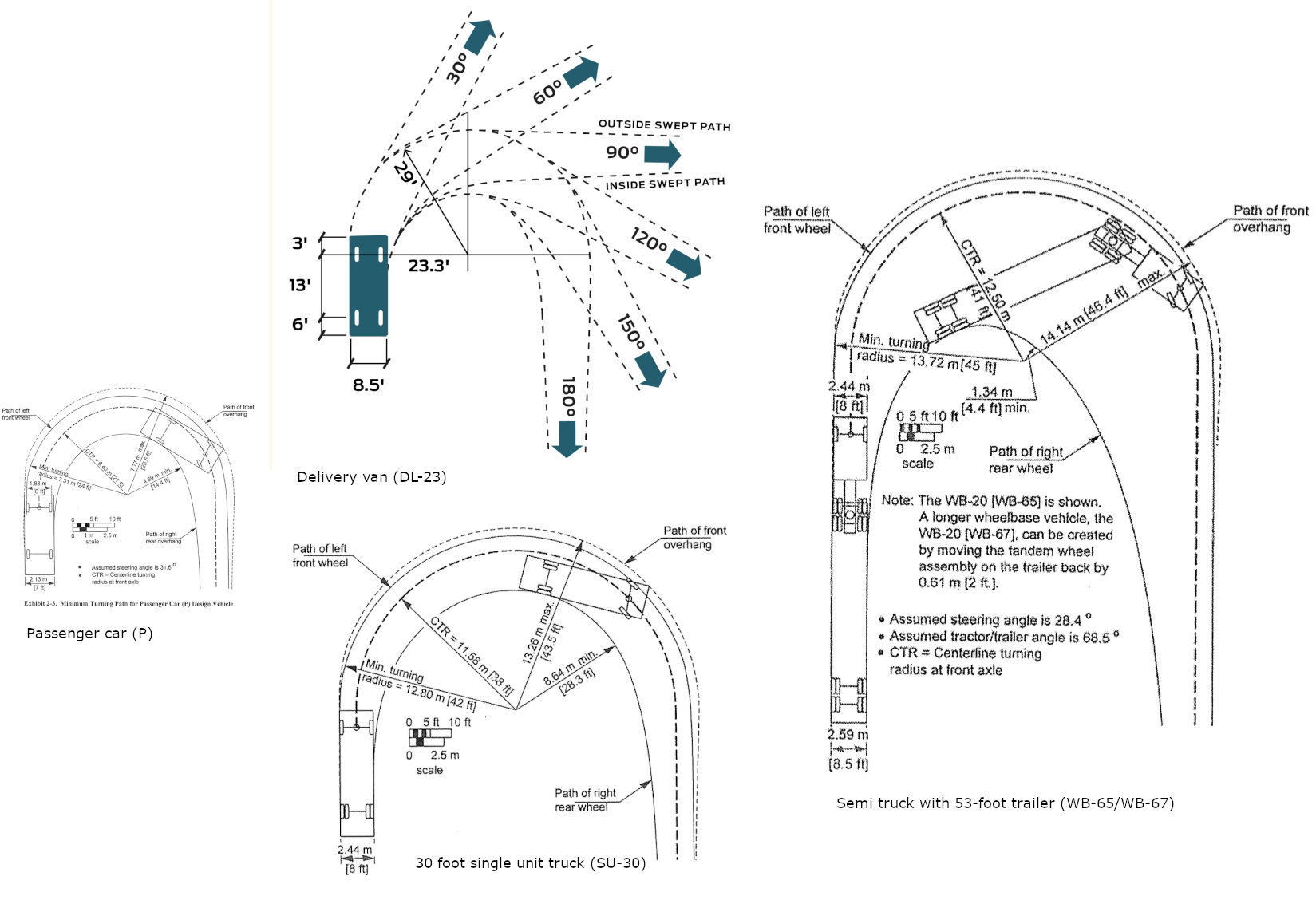
AASHTO Green Book, NACTO
Design vehicles and turning radii
- The larger the design vehicle, the larger the turning radius must be
- The larger the turning radius, the faster smaller vehicles will travel around the turn
Design vehicles in North Carolina
From the NCDOT roadway design manual (all state owned roads, emphasis mine)
North Carolina state law G.S. 20-115.1 allows vehicles with WB-62 and WB-62FL design characteristics on all North Carolina primary routes. Abide by the following guidance when selecting the design vehicle on all state routes.
- WB-62FL shall be the standard design vehicle for all primary routes in the state and should be considered on industrialized streets that carry high volumes of truck traffic or provide local access for large trucks. Primary routes are defined as any interstate, US, or North Carolina route.
- WB-62 shall be the standard design vehicle for all other routes, with context sensitive considerations given to constrained corridors.
Under special circumstances, the standard design vehicle may be larger than a WB-62FL when the project is in the vicinity of specialized trucking facilities or smaller than a WB-62 due to project constraints. If the standard design vehicle cannot be accommodated, discuss the project specific constraints with the project team and Division and develop documentation of the decision-making process. At minimum, accommodating a Conventional School Bus (S-BUS 36) should be considered. Coordinate with the local school system to determine if a Large School Bus (S-BUS 40) should be specified in lieu of the S-BUS 36.
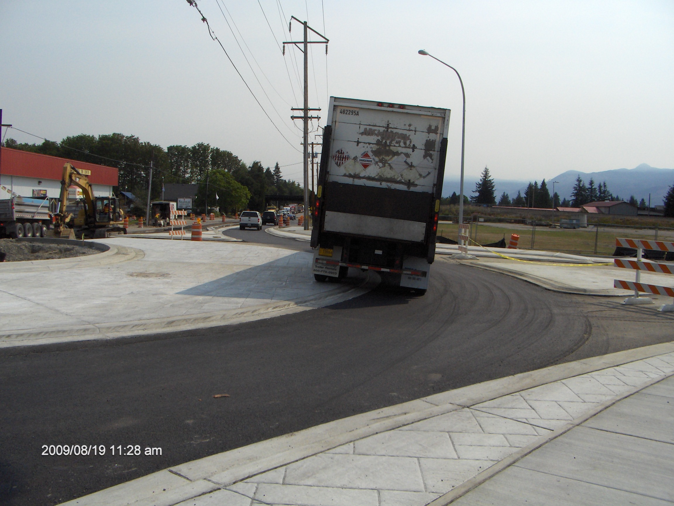
Introducing control vehicles
- The “control vehicle” is a newer concept, responding to the idea that we don’t need to design all our street for giant trucks
- The control vehicle is the largest vehicle that could get down the street, even if that meant crossing the center line, driving over some curbs, making a three-point turn, etc.
- E.g. we know that moving trucks may need to go down residential streets, but it doesn’t need to be easy
The managed vehicle
- The most common vehicle that uses a street
- The intersection should be designed to manage the turning speed of this vehicle
- e.g. keep turning speeds below 10mph at protected intersections
Mountable curbs and aprons: have your radius and eat it too
© WSDOT
Design speeds and speed limits
- Every road has a “design speed”
- This is the speed that the road is designed for, often higher than the speed limit
- Speed limits are usually set based on the 85th percentile speed
Risk compensation
- When you make a system safer, humans often behave more dangerously
- Roads with higher design speeds lead people to drive faster
- Safer cars lead to more dangerous driving
- Better armor and protective equipment leads soldiers to behave more dangerously
- The SawStop table saw stops automatically if it senses skin; they advertise they have saved 6,000 fingers with 80,000 saws sold. I don’t think 7.5% of non-SawStop saws have cut off someone’s finger…
The Tullock spike
- Gordon Tullock proposed the best way to improve road safety would be to mount a dagger in the center of every steering wheel
- This would make people drive so carefully crashes would be a thing of the past
Highway capacity analysis
- There are complex formulae for determining the capacity of a roadway, based on roadway design, driver behavior, signalization, access (entrances/exits/weaving), car/truck traffic composition, etc.
- Once capacity is determined, it is used to compute a level of service from A to F
Level of service
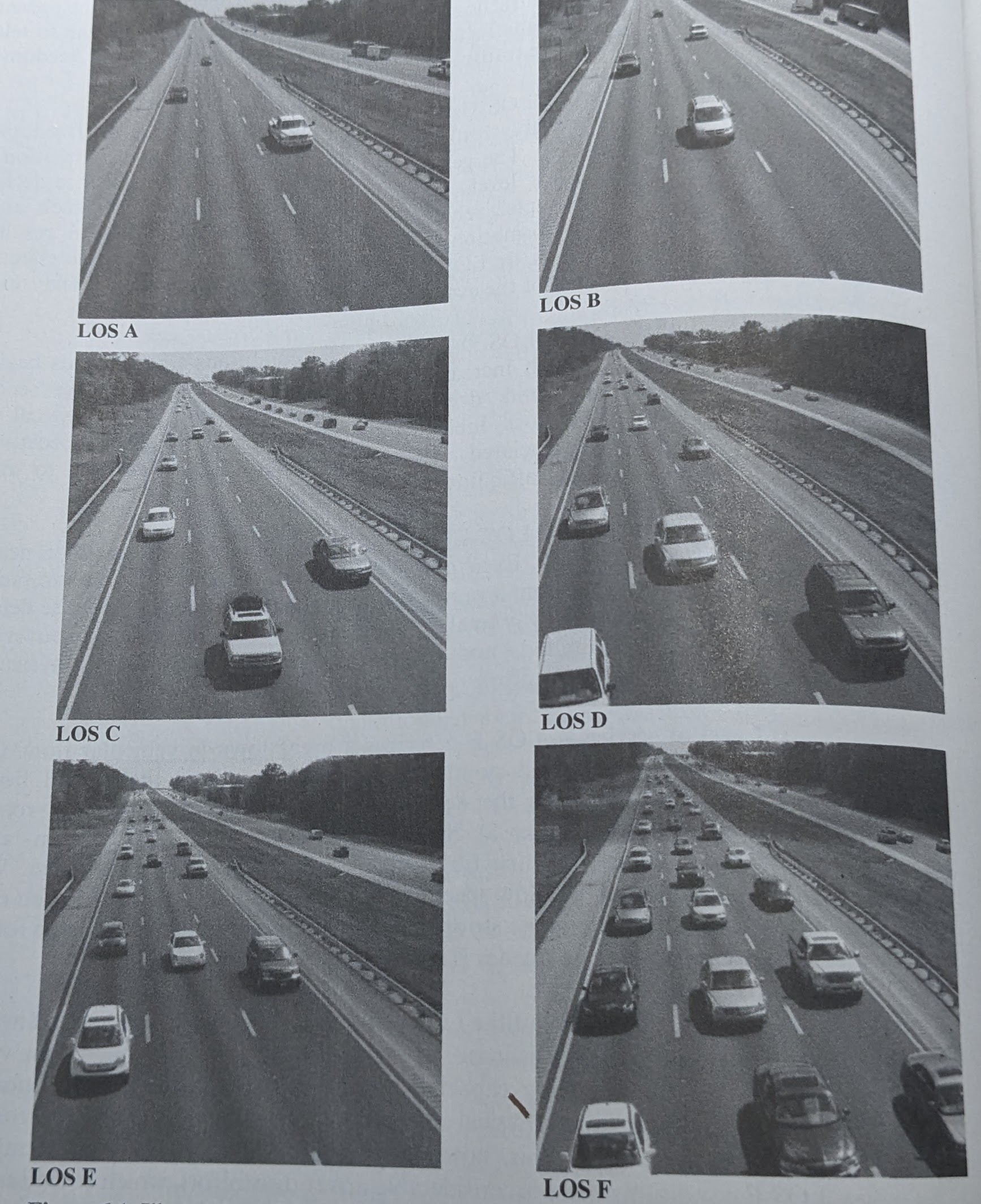
Mannering and Washburn (2020)
Level of service: intersections
- There is also an intersection LOS, based on seconds of delay for the average vehicle
LOS F ≠ failure
- Engineering guidance suggests maintaining at or above LOS D
- In urban areas, this is not going to be possible
- You will
sometimesalways get pushback on projects that worsen LOS, but it’s important to account for project context - LOS F shouldn’t be viewed as a failure of the system, but as a measurement of delay
- The most economically productive places (e.g. Manhattan) often have very low LOS
- Some places are moving away from LOS for this reason
- Similarly, it’s okay if volume is sometimes larger than capacity; this is inevitable in urban areas
Traffic counts
- Traffic counts are a primary data source for traffic engineering
- They can be manual, temporary and automated, or permanent and automated
- They are used to determine annual average daily traffic (AADT), which is the basis of many other traffic engineering concepts
Design volume
- Projected volumes are often based on demand during a “design hour”
- This is often the 30th or 50th busiest hour of the year
- The design hour volume is often estimated by multiplying the AADT by a factor known as the K-factor
- There is evidence that this K-factor is getting smaller post-pandemic (Bhagat-Conway and Zhang 2023)
The Manual on Uniform Traffic Control Devices (MUTCD)
- This is an FHWA publication that regulates the design and placement of signs, signals, and pavement markings
- It provides a consistent set of signs and signals that drivers can expect to see
- Deviating from these can be difficult
- e.g. the new HAWK crossing signals took a while to be accepted
Signal warrants
- The MUTCD has a list of “warrants” for when a signal is justified, based on
- Vehicular volume
- Pedestrian volume
- School crossing
- Crash experience
- Traffic flow
- Railway grade crossings
- Not absolute rules, but strong suggestions
The pedestrian warrant
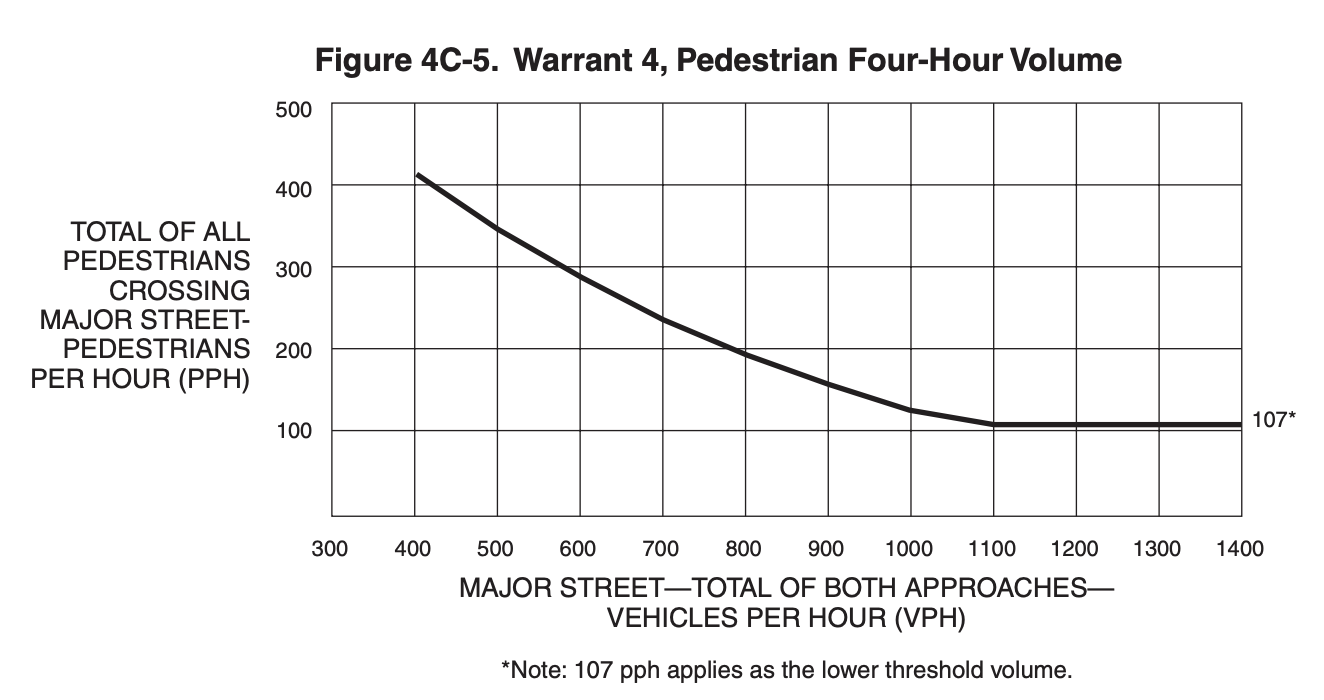
2009 MUTCD, rev. 3
The Pedestrian Volume signal warrant shall not be applied at locations where the distance to the nearest traffic control signal or STOP sign controlling the street that pedestrians desire to cross is less than 300 feet, unless the proposed traffic control signal will not restrict the progressive movement of traffic
Intersection control evaluation
- Intersection control evaluation is a systematic, multi-step process to consider the benefits and costs of traffic control devices
- Considers safety, capacity, and community context - though how is left up to implementers
- Used by 15 state DOTs, including NC
Signal timing
- Signal timing is a big part of traffic engineering
- The main concepts to remember are saturation flow, cycle length, lost time and effective red/green times
- The saturation flow is how much flow could occur from one direction, if that direction always had a green light
- The lost time is time that is lost due to acceleration, clearance times (when the signal is red all ways), etc.
- The effective green time is how long traffic coming from a direction is moving unimpeded
- It is not the same as the green time, because of the lost time
- A phase is a single set of movements
- Cycle length is the amount of time it takes for the signal to complete all phases
- The shorter the cycle length, the longer the lost time
Traffic signal timing cards

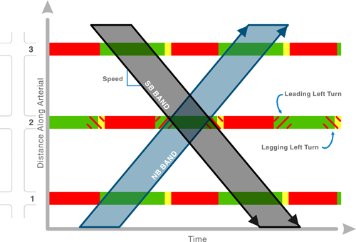
Time-space diagrams
The tension between planners and engineers
- There is often tension between engineers and planners
- Frequently, this stems from the more formulaic nature of engineering
- Some of the engineering formulae certainly do need changing, but understanding the professional environment in which engineers operate is helpful
References
Bhagat-Conway, Matthew Wigginton, and Sam Zhang. 2023. “Rush Hour-and-a-Half: Traffic Is Spreading Out Post-Lockdown.” PLoS One.
Mannering, Fred L, and Scott S Washburn. 2020. Principles of Highway Engineering and Traffic Analysis. 7th ed. Wiley.
Thanks to Kush Bhagat for insights on transportation engineering

This work by Matthew Bhagat-Conway is licensed under a Creative Commons Attribution 4.0 International License.
![]()