Economic analysis

Matt Bhagat-Conway

Planning and economic development

• Economic development is often a justification for planning activities
  • Employment, retail sales, tax base increases
• Economies are complex, linked, and have many feedback loops, so analyzing them can be challenging

Shift-share analysis

• Regional employment growth by industry can be divided into three components
  • National share: growth attibutable to the overall level of growth across all industries nationally
  • Industry mix: excess growth or decline in a particular industry nationally
  • Regional shift: excess growth or decline in a particular industry in this region

A shift-share analysis

• Let’s analyze the growth of the manufacturing industry in North Carolina since 2010
• All the data we’re using here comes from FRED

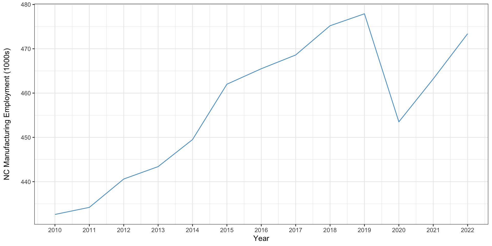
NC Manufacturing employment since 2010

• In 2010, total NC manufacturing employment was 433,000
• In 2022, it was 474,000
• The growth was 41,000 jobs or 9.5%

Breaking it down: national share

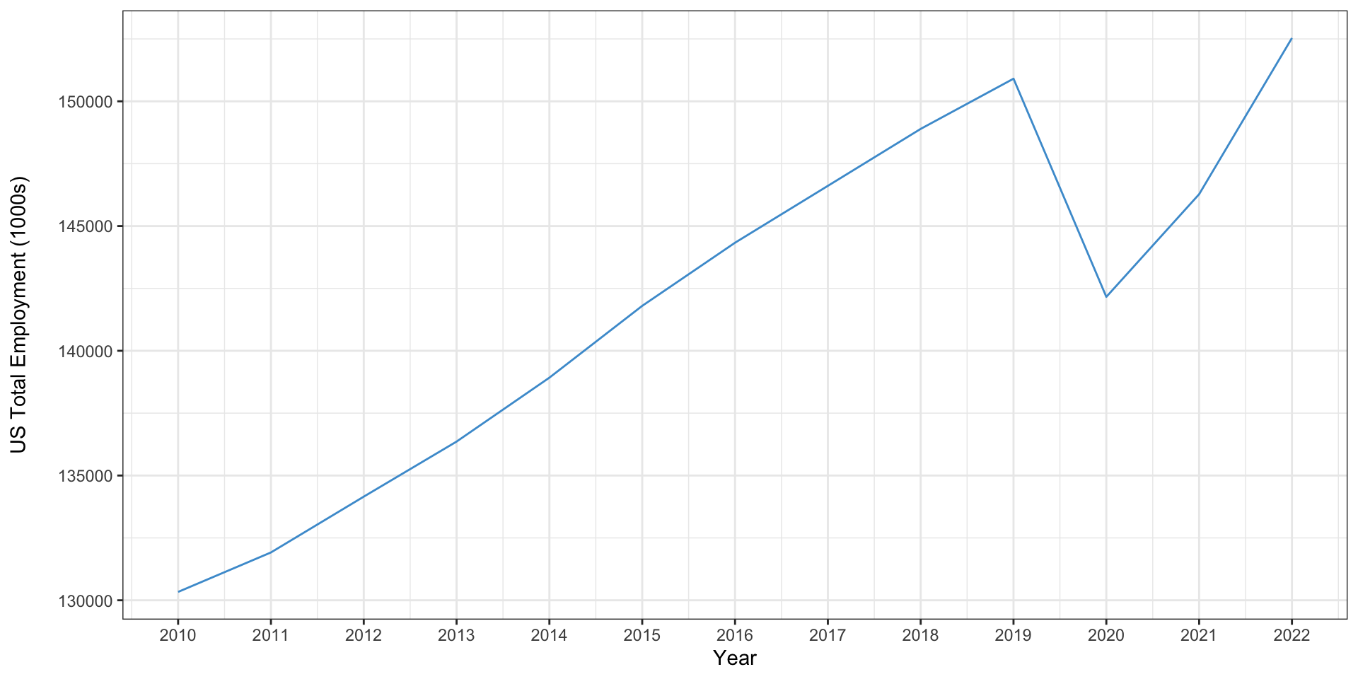
• In 2010, total US employment was 130 million
• In 2022 it was 153 million
• The growth rate was 17%
• If NC manufacturing had grown at the same rate as national employment, it would have grown by \(17\% \times 433,000 = 73,610\) jobs rather than 41,000

The industry mix

• Also known as “competitive share”
• Manufacturing has been declining in the US overall for some time
• The industry mix accounts for differences between the industry’s national growth rate and the national growth rate overall
• It is calculated as the national industry growth rate minus the national all-jobs growth rate, multiplied by the original employment, i.e.

\[ (G_{ind} - G_{all}) \times e_{ind,t=1} \]

where \(G_{ind}\) is the national growth rate of employment in this industry, \(G_{all}\) is the growth rate of national employment overall, and \(e_{ind,t=1}\) is employment in this industry at the start of the period

Calculating the industry mix

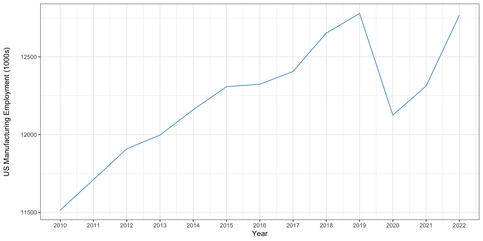
• US manufacturing employment was 11.5 million in 2010
• It was 12.8 million in 2022
• It grew 11%; growth across all industries was 17%
• What is the industry mix for manufacturing?
  • The difference in rates is -6%
  • \(-6\% \times 433,000 = -25,980\)

The influence of national trends

• If NC had followed national trends for manufacturing growth, it would have added 73,610 + -25,980 = 47,630 manufacturing jobs
• It actually added 41,000
• The rest is due to regional trends

Regional shift

• This measures the regional part of employment growth
• Is is calculated as the local growth rate of the industry minus the national growth rate, times the original employment in the industry

\[ (g_{ind} - G_{ind}) \times e_{ind,t=1} \]

where \(g_{ind}\) is the growth rate of the industry in the region.

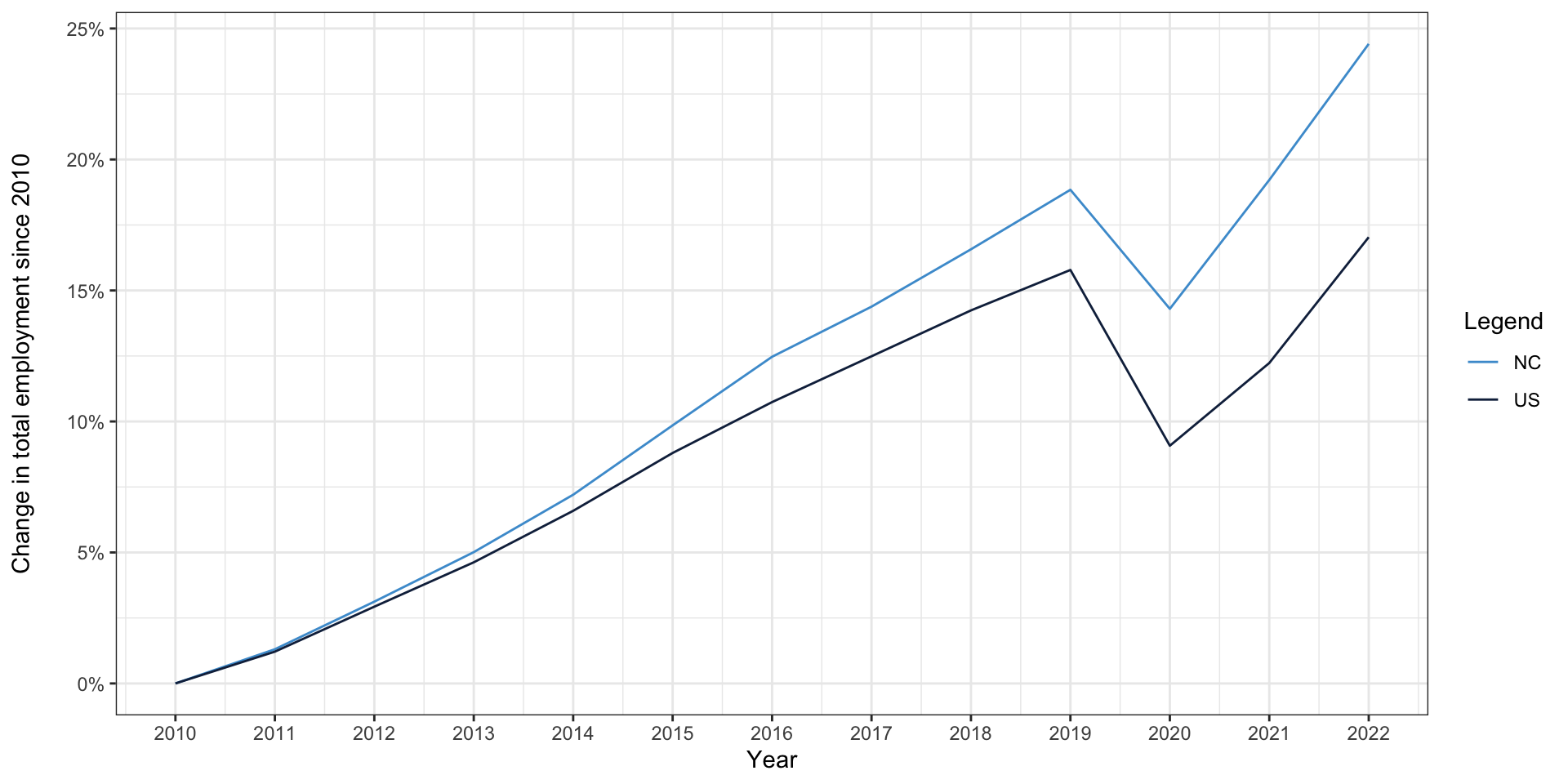
Calculating regional shift

• Manufacturing in NC grew at 9.5%, vs. 11% nationally, between 2010 and 2022
• The difference in rates is -1.5%
• This leads to a regional shift of \(-1.5\% \times 433,000 = -6,495\) jobs

Putting it all together: shift-share for NC manufacturing

• National share: 73,610
• Industry mix: -25,980
• Regional shift: -6,495
• Total: \(73,610 + -25,980 + -6,495 \approx 41,000\)

Interpreting shift-share

• The national share is just a measure of how well the national economy is doing overall, and is a kind of reference point for the other numbers
• The industry mix is a measure of how well an industry is doing relative to the overall economy
  • If positive, it’s doing better than the overall economy
  • If negative, it’s doing worse
• The regional shift is a measure of how well an industry is doing locally relative to that industry nationally
  • If positive, it’s growing faster locally than nationally
  • If negative, the reverse

What if the region overall is growing faster than the national average?

• This will contribute to higher regional shift in all industries
• Regional shift does not measure how well an industry is doing relative to other industries in the same region
• It measures how an industry in a region is doing relative to that industry nationally

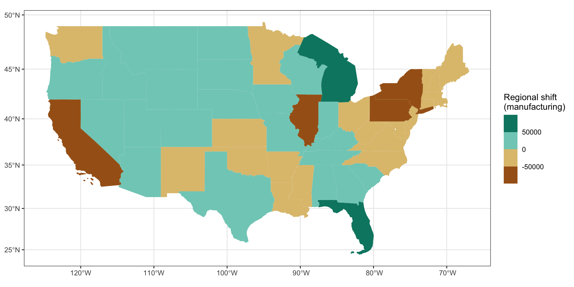
Where does manufacturing have a positive regional shift?

• I initially suspected NC would have a positive regional shift for manufacturing

Economic base theory

• Economic base theory divides employment into two categories: basic and non-basic
• Basic employment brings capital into the region, by serving demand elsewhere
  • e.g. natural resources exploitation, R&D, long-distance logistics, etc.
• Non-basic employment redistribute money within the region, by serving local demand
  • e.g. plumbers, electricians, grocery stores, etc.

The role of basic and non-basic employment

• Clearly, we need both types of employment
• But basic employment plays a special role, as it increases overall wealth
• Investments to increase basic employment increase the economic well-being of a region

The base multiplier

• An additional basic job will spur the creation of additional non-basic jobs
• The base multiplier is the ratio of non-basic to basic employment in a region
• It is assumed that an additional basic job will lead to this many total new jobs
• When you see analysis that says something like “this new investment will directly support 1000 jobs and indirectly support 800 more,” this is what they’re doing

The location quotient

• Generally, employment statistics aren’t broken out by basic or non-basic
• Instead, location quotients are used
• This is the ratio of the share of employment in an industry in a region to the share of employment in that industry nationally
• The idea is that the national average is what percent of employees need to be in that industry to serve local demand
• If the location quotient is above one, those excess workers are likely serving outside demand—the excess workers are basic employment
• If it is below one, that region is likely importing in that industry—all workers are non-basic employment

Calculating the location quotient

• 9.9% of workers in NC work in manufacturing (474,000), vs. 8.4% nationally
• The location quotient is \(\frac{9.9\%}{8.4\%} = 1.18\)
• How many of those jobs are basic? 🤔
• 15.2% or 71,818
• Where did 15.2% come from??
• \(\frac{0.18}{1.18}\)
• The one represents the non-basic employment, 0.18 the non-basic, and 1.18 the total

The location quotient in terms of jobs

• It may be easier to think about this in terms of total jobs
• If 8.4% of workers nationally are in manufacturing, we estimate 8.4% of North Carolina’s workers need to work in manufacturing to serve local demand, or 403,116
• There are 474,000 workers in manufacturing in NC
• 474,000 - 403,116 = 70,884 (slightly different due to rounding)

Problems with the location quotient

• It doesn’t account for local conditions
• For instance, there are a lot more snowplow operators in Wisconsin than Florida
  • And this has nothing to do with export of snow removal services from Wisconsin to Florida

Deriving base multipliers from location quotients

• If you calculate location quotients for every industry, you can estimate total basic and non-basic employment
• This can be used to derive the base multiplier
• On average, this is how many non-basic jobs are associated with each basic job
• It’s not going to be a perfect predictor of new non-basic jobs
  • Different types of basic jobs will drive different amounts of non-basic growth
  • Economies of scale may reduce need for per-capita non-basic employment in some sectors
  • Though that may drive growth in others…

Input-output models

• The other tool commonly used for economic impact analysis is an input-output model
• In the US, the IMPLAN software is ubiquitous, so you may also see this referred to as an IMPLAN model

Input-output models: theory

• Every industry produces some level of output
• Three things can happen to those outputs
  • They can be purchased by consumers
  • They can be exported
  • They can be used as inputs to other industries
    • This is the key insight behind the input-output model

Input-output models

• The output of each industry is the sum of demands from consumers, exports, and demands from other industries
• So, for each industry, we have a function like this (using notation from Miller and Blair (2009))

\[ x_i = z_{i1} + z_{i2} + \cdots + z_{ij} + f_i \]

where

• \(x_i\) is the output of industry \(i\) (usually in dollars)
• \(z_{ij}\) is the amount of industry \(i\)’s goods demanded by industry \(j\), and
• \(f_i\) is the final demand for the output of industry \(i\) (consumer demand + exports)

Input-output matrix

• We can put these functions into a matrix for every industry, showing all interindustry relationships

\[\begin{align*} x_1 & = z_{11} + z_{12} + \cdots + z_{1n} + f_1 \\ x_2 &= z_{21} + z_{22} + \cdots + z_{2n} + f_2 \\ \vdots \\ x_{n} & = z_{n1} + z_{n2} + \cdots + z_{nn} + f_n \end{align*}\]

• The rows are the total outputs of each industry as a function of the demand from other industries and consumers
• What about the columns?

Interpreting input-output matrices

• The columns are the inputs to each industry
• If we sum up a column of \(z\) s, we get the total value of inputs to that sector to produce a given output
• Remember these are all in dollars
• Are the outputs of an industry equal to the inputs in dollar value?

Payments

• What goes into the difference between output value and input value?
  • Imports from outside the region
  • Labor
  • Capital
  • Land
  • Profit
  • Together referred to as “payments”

The full input-output model

• We can add terms for these, and create the full input-output model

\[\begin{matrix} z_{11} & z_{12} & \cdots & z_{1n} & f_1 &|& x_1 \\ z_{21} & z_{22} & \cdots & z_{2n} & f_2 &|& x_2\\ \vdots & \vdots & \ddots & \vdots & \vdots &|& \vdots \\ z_{n1} & z_{n2} & \cdots & z_{nn} & f_n &|& x_n \\ l_1 & l_2 & \cdots & l_n & \\ n_1 & n_2 & \cdots & n_n & \\ m_1 & m_2 & \cdots & m_n & \\ \hline x_1 & x_2 & \cdots & x_n \\ \end{matrix}\]

where

• \(l_i\) is the labor input to industry \(i\)
• \(n_i\) is other payments (rent, profit, etc.)
• \(m_i\) is imports

Using the input-output model

• We can add terms for these, and create the full input-output model

\[\begin{matrix} z_{11} & z_{12} & \cdots & z_{1n} & f_1 &|& x_1 \\ z_{21} & z_{22} & \cdots & z_{2n} & f_2 &|& x_2\\ \vdots & \vdots & \ddots & \vdots & \vdots &|& \vdots \\ z_{n1} & z_{n2} & \cdots & z_{nn} & f_n &|& x_n \\ l_1 & l_2 & \cdots & l_n & \\ n_1 & n_2 & \cdots & n_n & \\ m_1 & m_2 & \cdots & m_n & \\ \hline x_1 & x_2 & \cdots & x_n \\ \end{matrix}\]

• Summing rows gives us total outputs
• Summing columns gives us total inputs
• The outputs of industry \(i\) are equal to its inputs

Applications of the input-output model

• Input-output models are often used in forecasting
• Here, it is hypothesized that something (usually final demand) changes
• We then use our input-output table to determine the ripple effects of that change through the economy
• When forecasting increased final demand, it’s important to differentiate new demand from displaced demand (see also Crompton 2006)
  • e.g., ticket sales at a stadium to people coming from outside the region are new demand
  • but ticket sales to locals may be displaced from other things (lower demand for other entertainment options)

Economic development and investment

As North American cities vie for the chance to be chosen by Amazon as the home of its second headquarters, one Georgia city has stepped up to the plate. The city council of Stonecrest, Georgia voted 4 to 2 on Monday to change its name to Amazon, Georgia and give the company 345 acres of land if Amazon selects it as the HQ destination, according to local media.

Shannon Liao/The Verge

Analyzing economic development and investment

• From looking at base multipliers and the input-output model, we can see why cities might want to attract economic development
• Often this takes the form of tax breaks, incentives, etc.
• This can be economically valuable, but it’s common to overstate benefits (O’Flaherty 2005)
• A key consideration is opportunity cost
  • We can’t consider all the economic activity brought to a city as the benefit
  • We have to consider what else could have been done with the economic development dollars
• Jobs are only a benefit in the amount they pay more than whatever else the employees could be doing
• Land price increases are often touted as a benefit, but they aren’t—they’re just a transfer from renters or future landowners to current landowners
  • Of course, if the future landowners are bringing money from out of town, that may increase local wealth

Pareto improvements

• We’ve talked a lot about counting money from outside the region as economic development
• As you increase the size of your region, this becomes harder to do
• For economic development to be optimal, the benefits to the place receiving the development must exceed the costs to the place losing the development
• If all actors have perfect information, act completely rationally, and are completely flexible in negotiations, this will always be true (O’Flaherty 2005)
• If they don’t, however, economic development policies (or lack thereof) may ultimately cost more than they benefit
  • And they don’t…

References

Crompton, John L. 2006. “Economic Impact Studies: Instruments for Political Shenanigans?” Journal of Travel Research 45 (1): 67–82. https://doi.org/10.1177/0047287506288870.

Miller, Ronald E., and Peter D. Blair. 2009. Input-Output Analysis: Foundations and Extensions. 2nd ed. Cambridge University Press.

O’Flaherty, Brendan. 2005. City Economics. Harvard University Press. https://doi.org/10.4159/9780674041615.

This work by Matthew Bhagat-Conway is licensed under a Creative Commons Attribution 4.0 International License.