| 136,000 | 34,000 | 18,440 | 12,000 | 151,000 | 50,000 | 17,041 | 119,682 | 0 | 71,682 |
| 129,200 | 151,400 | 24,000 | 10,000 | 0 | 21,901 | 98,000 | 167,000 | 62,000 | 164,000 |
| 0 | 4,020 | 46,841 | 2,041 | 23,000 | 35,904 | 45,000 | 358,211 | 0 | 95,300 |
| 109,000 | 151,000 | 53,019 | 0 | 4,082 | 37,000 | 28,500 | 21,191 | 0 | 36,000 |
| 26,941 | 74,733 | 87,050 | 55,000 | 175,250 | 140,000 | 155,000 | 77,000 | 58,000 | 75,000 |
Statistics I: Descriptive statistics
Matt Bhagat-Conway
What is statistics
- At its heart, statistics is a tool to summarize data into actionable information
- Statistics can describe the current situation, forecast future outcomes, and understand relationships between variables
- Algebra and calculus are math with too few numbers, statistics is math with too many
Descriptive vs. inferential statistics
- Descriptive statistics describe patterns in data
- Inferential statistics are focused on statistical “tests” to determine if data are consistent with hypotheses
- Descriptive statistics are the most common in planning
Statistical data
- Many consistent observations
- Generally numerical
- Representative (more on that below)
Measures of central tendency
- The most common statistics are measures of central tendency
- These statistics describe a dataset with a single number representing the center of the dataset
Measures of central tendency
Suppose we have data on incomes for 50 households in NC.
What is the income for a typical household in NC?
Distributions and histograms
Distributions and histograms
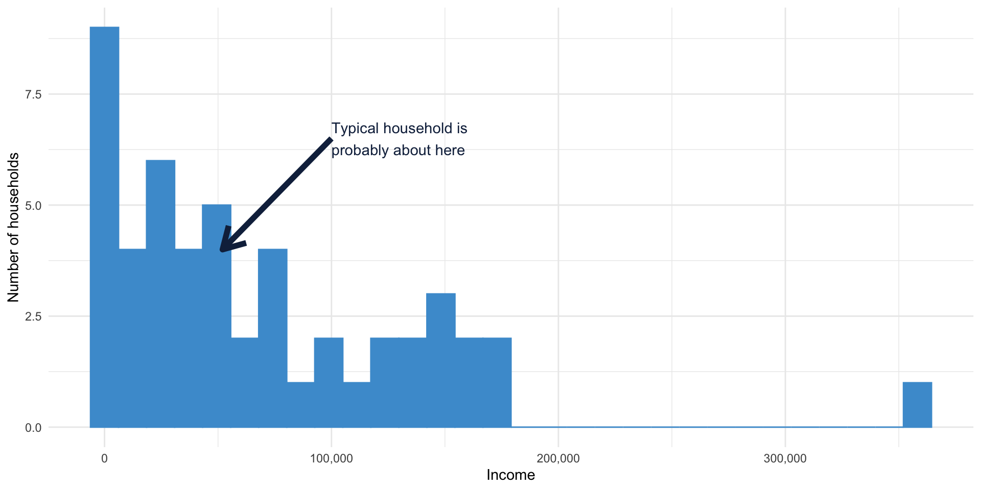
What does “typical” even mean?
The mean
- Most common measure of central tendency
- The income everyone would have if income were evenly distributed
The mean
- Add up all the incomes
- Divide by the number of households
The mean
\[ \bar x = \frac{x_1 + x_2 + \cdots + x_n}{n} \]
or
\[ \bar x = \frac{\sum\limits_{i=1}^n x_i}{n} \]
Calculating the mean of our data
Let’s calculate the mean of the sixth column of our data
50,000 + 21,901 + 35,904 + 37,000 + 140,000 = 284,805
284,805 / 5 = 56,961.0
Calculating the mean of our data
Now, calculate the mean of the first column:
136,000; 129,200; 0; 109,000; 26,941
80,228
Don’t do it this way
- It’s totally fine if this is the last time you calculate a mean by hand
- Let’s calculate the mean of all 50 households, but let’s use Excel
- Download the Excel file from Canvas
Means in Excel
- Excel has many functions for calculating values
- You enter these by having a cell start with
= - To calculate a mean, you use the
AVERAGEfunction - You can specify a range of values with a
: - For example, to calculate the mean of the first five values in the data, enter in an empty cell:
=AVERAGE(A2:A6)
Means in Excel
- Calculate the mean of all 50 income values
=AVERAGE(A2:A51)
68,228.58
Means can be wonky
All of these are true:
- The average American has 1.006 skeletons
- The average starting salary for UNC Geography majors graduating in 1986 was $250,000 ($728,000 today)
- The average American president has spent two seconds in a high-radiation area cleaning up after a nuclear meltdown
Why? Outliers
- Very large or very small values have a strong effect on the mean
- Because of how the mean is calculated, very large values are distributed over all observations
Why? Outliers

The median
- The median is the middle number in a set of numbers
- The median is much less sensitive to outliers, because it is based on the numbers in the middle rather than all the numbers

Calculating the median
- Sort the numbers
- If there are an odd number of observations => find the middle one
- If there are an even number of observations => take the mean of the two in the middle
Calculating the median
50,000; 21,901; 35,904; 37,000; 140,000
21,901; 35,904; 37,000; 50,000; 140,000
Is the median higher or lower than the mean?
Exercise: outliers
- What happens to the mean and median if the household making $140,000 makes some good investments and now makes $500,000?
Exercise: computing the median
Now, calculate the median of the first column:
136,000; 129,200; 0; 109,000; 26,941
109,000
Computing the median in Excel
- Calculate the median of all 50 income values
=MEDIAN(A2:A51)
48,420.50
The incomes are all whole numbers. How can the median end in .50?
When to use medians
- Generally, any dataset likely to have outliers
- Commonly used for
- Income
- Housing prices
Applications of the median in planning
- Most common is probably area median income (AMI)
- This is the median income in a metropolitan area or county
- Used to determine eligibility for many federal assistance programs
- For instance, some housing programs are restricted to those below 80% or 50% of Area Median Income
The relationship between the median and the mean
- The mean will be pulled in the direction of any outliers
- So, in a datset with large outliers, the mean will be higher than the median (e.g. income)
- Opposite in a dataset with small outliers (e.g. age at cancer diagnosis)
Percentiles: a more general median
- 50% of observations are above and 50% are below the median
- We could also calculate the value 20% of the observations are below
- This would be the 20th percentile
Calculating percentiles
What is the 20th percentile of this list of incomes?
50,000; 21,901; 35,904; 37,000; 140,000
21,901; 35,904; 37,000 50,000; 140,000
Percentiles and outliers
- Are low or high percentiles sensitive to outliers?
Calculating percentiles
- Percentiles might fall between two numbers
- For instance, what is the 30th percentile of these five incomes?
50,000; 21,901; 35,904; 37,000; 140,000
Calculating percentiles
- No single agreed-upon method
- A straightforward method is to find the value where no more than p% of values are less than, and no less than p% are less than or equal to
- More complex methods interpolate between nearby values
- In large samples, all methods will give similar results
Calculating percentiles
What is the 30th percentile of this list of incomes?
50,000; 21,901; 35,904; 37,000; 140,000
| Percentile | Value |
|---|---|
| 20 | 21,901 |
| 40 | 35,904 |
| 60 | 37,000 |
| 80 | 50,000 |
| 100 | 140,000 |
Calculating percentiles
- Excel has two percentile functions,
PERCENTILE.INCandPERCENTILE.EXC - Both interpolate percentiles, and differ slightly in how they calculate percentiles
- In large samples, they will be similar
PERCENTILE.EXC vs PERCENTILE.INC
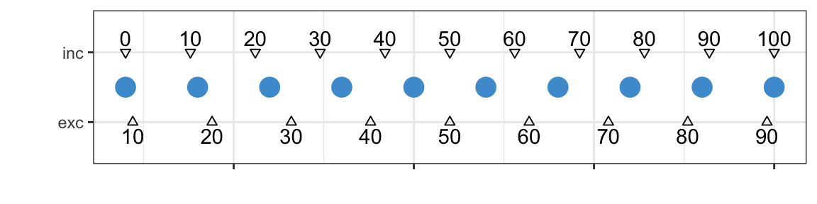
- Way more information than you ever wanted on percentile calculation: Hyndman and Fan (1996) 😱
PERCENTILE.INCis a “type 7” percentile, andPERCENTILE.EXCis a “type 6” 😱 😱
Calculate the 20th percentile of income in Excel
=PERCENTILE.INC(A2:A51, 0.2)
or
=PERCENTILE.EXC(A2:A51, 0.2)
Uses of percentiles
- Percentiles are often used when evaluting equity
- Percentiles are used in hypothesis tests
- Percentiles are used to find outliers
- Percentiles are used to calculate the interquartile range
The mode
- The mode is just the most common value in a dataset
- Can be misleading with continuous data
The mode
What is the mode of the NC income data?
| 136,000 | 34,000 | 18,440 | 12,000 | 151,000 | 50,000 | 17,041 | 119,682 | 0 | 71,682 |
| 129,200 | 151,400 | 24,000 | 10,000 | 0 | 21,901 | 98,000 | 167,000 | 62,000 | 164,000 |
| 0 | 4,020 | 46,841 | 2,041 | 23,000 | 35,904 | 45,000 | 358,211 | 0 | 95,300 |
| 109,000 | 151,000 | 53,019 | 0 | 4,082 | 37,000 | 28,500 | 21,191 | 0 | 36,000 |
| 26,941 | 74,733 | 87,050 | 55,000 | 175,250 | 140,000 | 155,000 | 77,000 | 58,000 | 75,000 |
0
Measurement levels
- Nominal/categorical: categories with no order (e.g. colors)
- Ordinal: ordered categories with no information about distance between them (e.g. much less, less, same, more, much more)
- Interval: distances between items are meaningful, ratios are not (no meaningful zero; e.g. temperature)
- Ratio: distances between items and ratios are meaningful (e.g. income)
- Modes are most useful for nominal and ordinal data
Mode of categorical data
| Manager, Professional Administrator | Sales, retail |
| Manager, Professional Administrator | Transportation operator |
| Other Service | Unemployed |
Manager, professional administrator
Measures of dispersion
- So far, we’ve looked at measures of the center of a dataset
- But what about measures of how spread out a dataset is?
Measures of dispersion
- There is another dataset in the second tab of the Excel sheet
- This has another sample of 50 households, but all have a household member 30–31 years old
- Calculate the mean income for this sample
- 30-31: 71,819
- Overall: 68,229
Dispersion
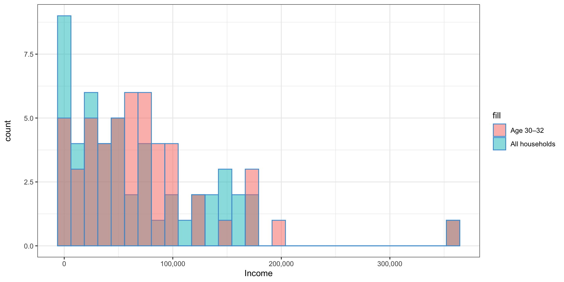
- Both have similar means, but the 30–31 year olds’ income is less spread out
Aside: squares and square roots
- The square of a number is just that number times itself
- Also the area of a square with sides of that length
- The square root of a number is the reverse: whatever other number squared equals that number
- Also the length of the sides of a square with that area
- The square is always positive, even when the number is negative
Variance and standard deviation
- The variance is a measure of how spread out the data are
- For each observation, subtract the mean
- Square the results
- Sum them up
- Divide by the sample size minus 1
Variance and standard deviation
\[ Var(x) = \frac{\sum\limits_{i=1}^{n}(x_i - \bar x)^2}{n - 1} \]
Why do we divide by \(n-1\) and not \(n\)?
- Because \(\bar x\) is estimated from our data, it is probably a little closer to our data than the true \(\bar x\) would be if we had every data point
- Because we used up one degree of freedom calculating \(\bar x\) 😱
- Basically, if you know all but one of the data points, and the mean, you can figure out the last data point
- So there’s actually \(n - 1\) independent data points once you calculate the mean
Variance and standard deviation
50,000; 21,901; 35,904; 37,000; 140,000
Calculate the mean: 56,961
Subtract the mean from each observation: -6,961; -35,060; -21,057; -19,961; 83,039
Square them: 48,455,521; 1,229,203,600; 443,397,249; 398,441,521; 6,895,475,521
Add them up: 9,014,973,412
Divide by the sample size minus one (4): 2,253,743,353
What are the units?
- How can the variance be 2.2 billion when the largest income is $140,000?
- Let’s follow the math
- Calculate the mean: the mean is in dollars
- Subtract the mean: the difference is in dollars
- Square the difference: the units are now dollars squared
The standard deviation
- The standard deviation is just the square root of the variance
- This way, the dispersion is expressed in the same units as the observations
- What is the standard deviation of our sample data? The variance was 2.25 billion
- 47,474
- The standard deviation is far more commonly used than the variance
What does the standard deviation actually mean?
- Kinda like how far the average observation is from the mean
- That actually has its own name: mean absolute deviation, \(\frac{\sum_{i=1}^n \lvert x_i - \bar x \rvert}{n}\)
- In the standard deviation, we square the differences instead of taking the absolute value
- This emphasizes outliers more heavily
- The standard deviation has a continuous derivative 😱
Calculating the standard deviation in Excel
- The Excel function
STDEVcalculates the standard deviation - Calculate the standard deviation of the two data sets
- NC dataset: 68,883
- Age 30–31 dataset: 63,489
- Which has the smaller standard deviation?
- Is this consistent with our expectations?
The interquartile range
- The standard deviation is by far the most common measure of dispersion
- The other common measure is the interquartile range
- This is just the 75th minus 25th percentiles
- It is mostly used in making boxplots
Hyndman, Rob J, and Yanan Fan. 1996. “Sample Quantiles in Statistical Packages.” The American Statistician 50 (4): 361–65.
![]()