Probability, distributions, and hypothesis tests

Matt Bhagat-Conway

What is probability?

• A representation of the likelihood of an event, between 0 and 1
  • 0=event will not happen, 1=event will happen, 0.5 = 50% chance event will happen

What is probability?

• A fair coin has a probability of 0.5 of coming up heads
• If you flip the coin many times, approximately 50% of the time it will come up heads

Logic rules for probability

• A and B are events (e.g. A is heads and B is tails)
• If A and B are mutually exclusive, the probability of A or B happening is just the sum of the probabilities of A and B

What does this have to do with means and standard deviations?

• Means and standard deviations are ways of describing a probability distribution
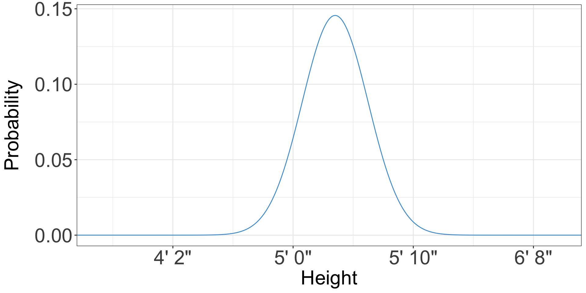
• A probability distribution describes how likely different values are
• For instance, height is approximately normally distributed

What does a probability of a height even mean?

• You likely know how tall you are
  • (if not, it’s conveniently written on your driver’s license/ID)
• There’s not a 10% or 50% or whatever chance than I’m 5’10”, I just am

Sampling

• Probability distributions are mostly meaningful when talking about a group
• I know how tall I am, but how tall is a random person picked from the class?
• That is what a probability distribution describes

Probability distributions

• The x axis is whatever your variable is
• The y axis is the probability of observing that value*

Probability distributions

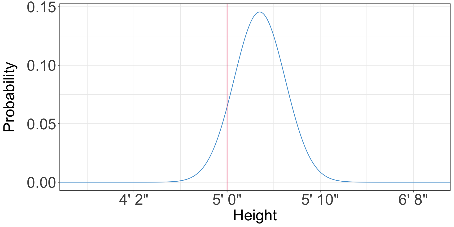
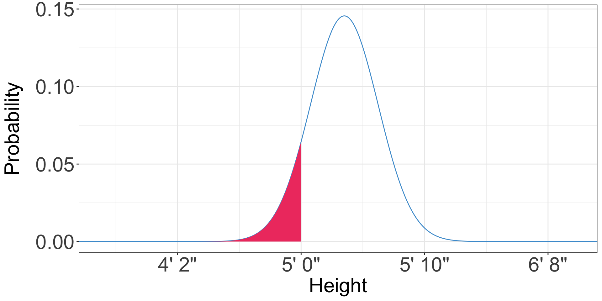
• What is the probability that a randomly chosen American woman is 5 feet tall?
  • 0.06

Probability distributions

• Is anybody likely to be exactly 5 feet tall, not 5 feet 1/128th inch or 4 feet 127/128th inch?

Probability distributions

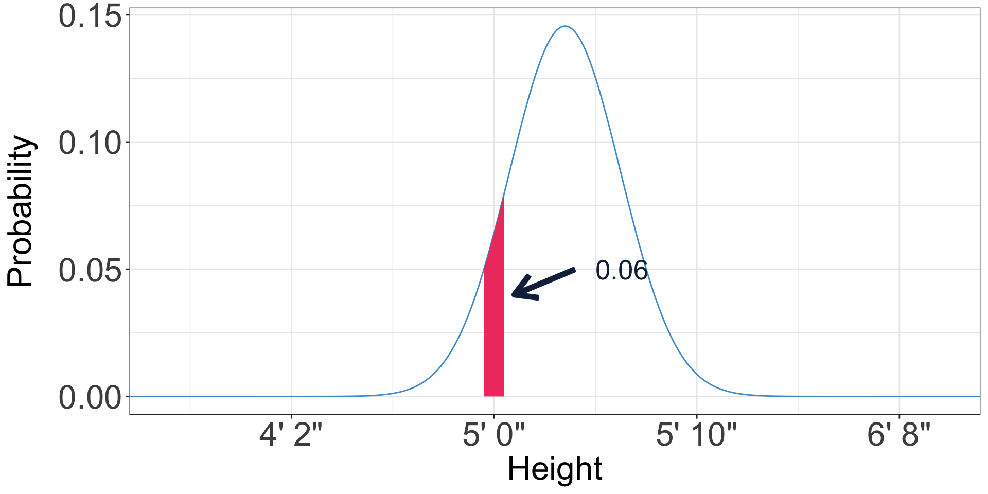
• We can only define the probability for a range of heights, for instance 4’ 11-1/2” to 5’ 1/2”
• The probability of any range is the area of the probability distribution in that range
  • If you’ve taken calculus, you might call this an integral
• The area under the entire distribution is 1 - because everyone has a height

Probability distributions

• The distribution we’ve been looking at is the normal distribution
• In a normal distribution, probabilities asymptotically approach 0 as you get further from the mean
  • i.e. they get close but never get there
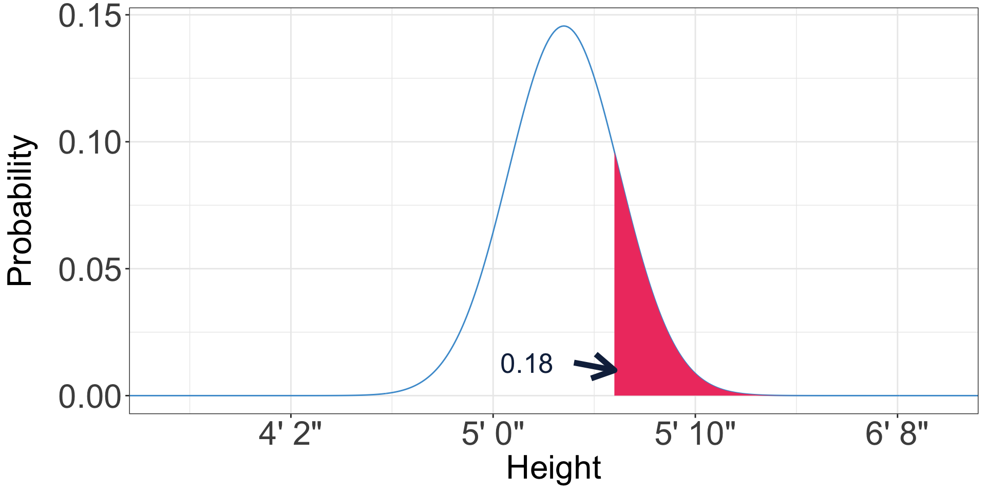
• When calculating probability, we most often are interested in the tails of the distribution
• For instance, what proportion of US women are over five feet six inches?

What proportion of US women are over five feet six inches?

Means, standard deviations, and the normal distribution

• Just like a set of data, distributions have means and standard deviations

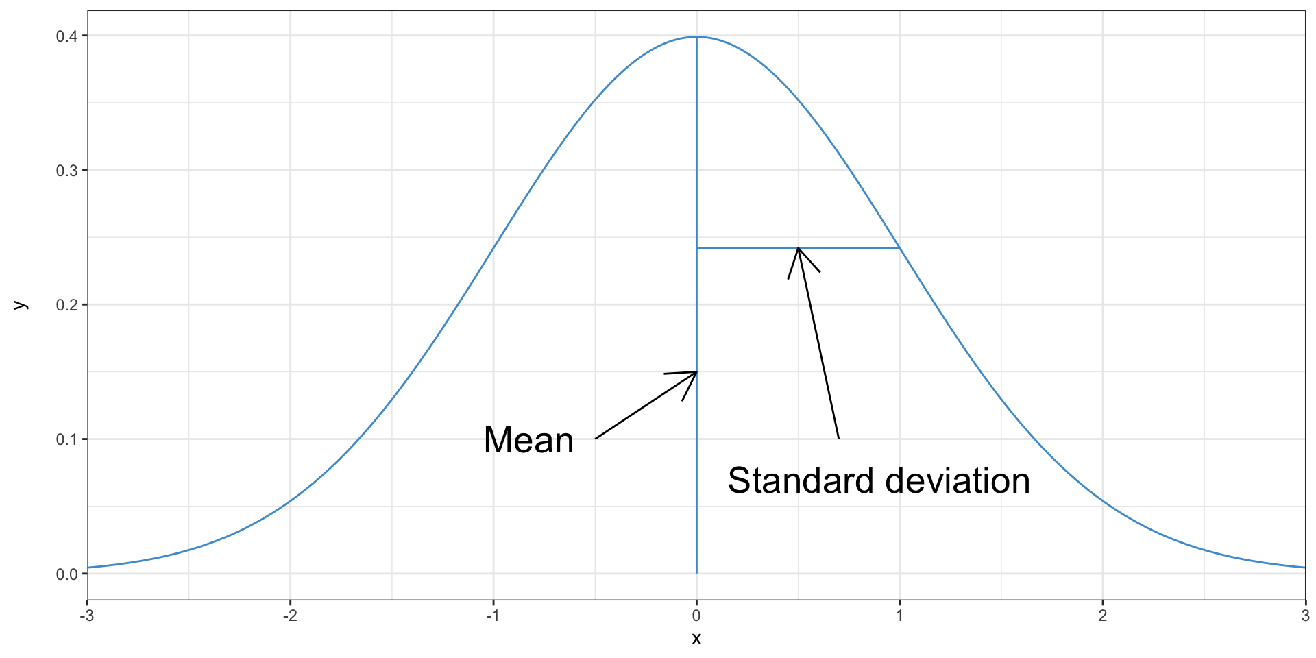
Means, standard deviations, and the normal distribution

• The mean and the standard deviation are the parameters of a normal distribution
• If you know them, you can figure out the rest of the distribution

Calculating probabilities from the normal distribution

\[ \Phi (x, \mu, \sigma) = \frac{1}{\sigma \sqrt{2 \pi}} e^{-\frac{1}{2}(\frac{x - \mu}{\sigma})^2} \]

jk use a computer

Calculating probabilities from the normal distribution

• Excel provides the NORM.DIST function to calculate probabilities from normal distributions
• The height of US women is normally distributed with mean 63.5 inches and standard deviation 2.74 inches
• =NORM.DIST(60, 63.5, 2.74, TRUE) is the probability that an American woman is 5 feet (60 inches) or less

Calculating probabilities from the normal distribution

• =NORM.DIST(60, 63.5, 2.74, TRUE) is the probability that an American woman is 5 feet (60 inches) or less
• This is a cumulative probability—i.e. it sums up all of the area under the normal distribution up to 5 feet

Calculating probabilities from the normal distribution

• What is the probability than an American woman is less than five foot six?

• 0.82

Calculating the other tail

• Excel only has this function for a cumulative normal distribution
• How would we estimate the probability an American woman is over five foot six?
• All probabilities must sum to one
• The probability that an American woman is less than five foot six is 0.82
• So the probability that an American woman is more than five foot six is 1 - 0.82 = 0.18

Calculating the other tail

Calculating the other tail

• What is the probability an American woman is more than five foot eight (68 inches)? . . .
• 0.05

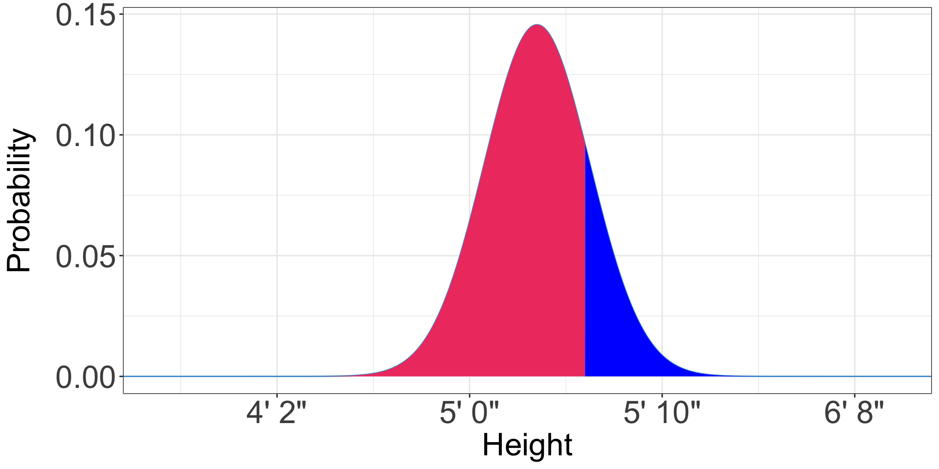
Calculating the middle

• What is the probability an American woman is between five feet (60 inches) and five foot six (66 inches)?

Calculating the middle

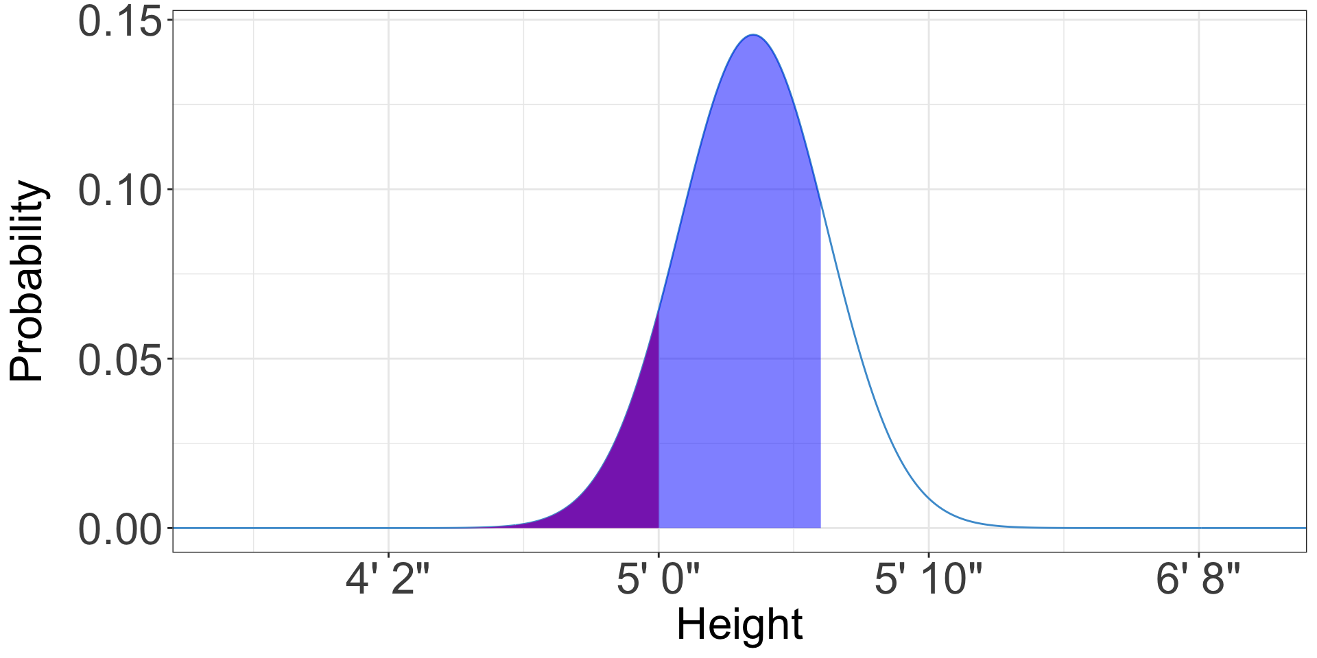
Calculating the middle

• What is the probability an American woman is between five feet (60 inches) and five foot six (66 inches)?
• We can subtract the probability an American woman is less than five feet from the probability she is less than five feet six
• Probability she is less than five foot six (66 inches): 0.82
• Probability she is less than five feet (60 inches): 0.1
• Difference: 0.72

Properties of the normal distribution

• If (you assume) your data are normally distributed, you can do a bunch of cool stuff with the normal distribution
  • In normally-distributed data, 95% of the data are within 1.96 standard deviations of the mean
  • 90% are within 1.645 standard deviations

Other distributions

• Many things in planning aren’t normally distributed
  • e.g., income is lognormal, city size is Zipf-distributed
• But the normal distribution (and its cousin the \(t\)-distribution) is still the most useful for hypothesis tests, which is mostly what we use distributions for in planning

The lognormal distribution

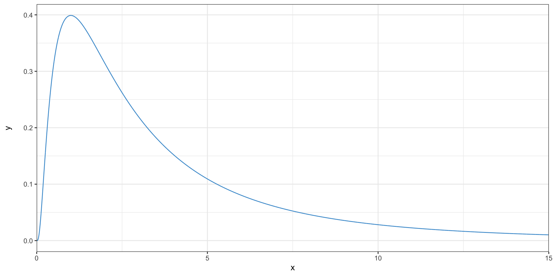
• This distribution is right-skewed
• It is called lognormal because the logarithms of the observations are normally distributed

The lognormal distribution

• Where are the outliers in this distribution?
• Is the mean higher or lower than the median?

The Zipf distribution

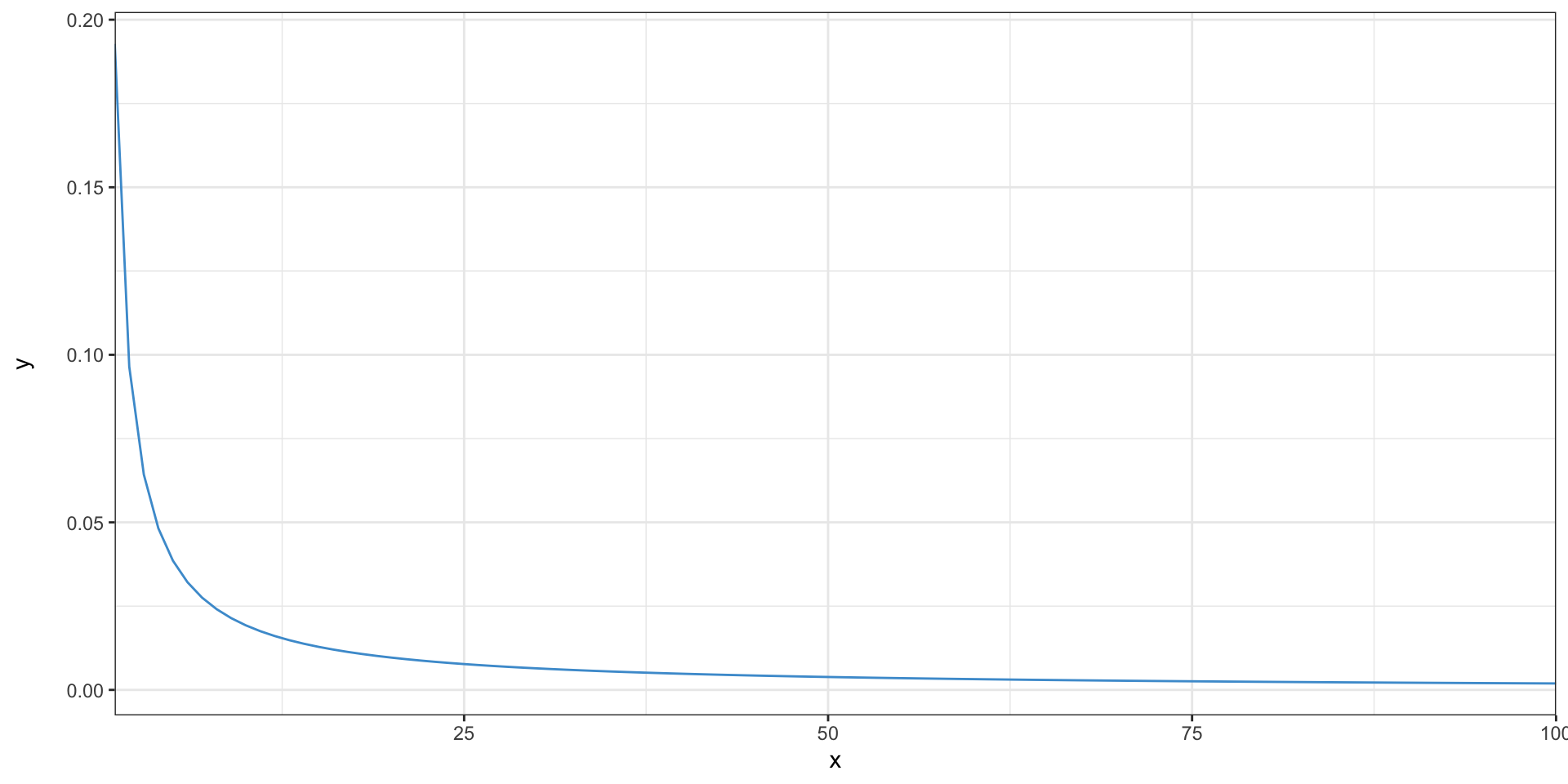
• The second biggest city is half as big as the first, the third is one-third as big, etc.

The Zipf distribution

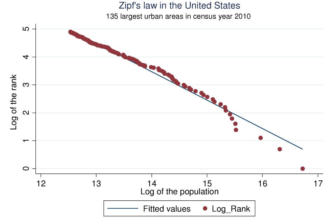
Arshad, Hu, and Ashraf (2018)

Samples and populations

• The sample is the data you have
• The population is everyone/everything you’re surveying
• The population distribution describes the probability of getting a person of a given height when you choose randomly from the population

Samples and populations

Sampling

• We almost never have a population
  • The Census and some administrative data are exceptions, or close to it
• A key goal of statistics is to allow use to use knowledge from samples to make conclusions about the full population
• Sampling theory deals with how statistics based on a sample are related to parameters of the full population

Sampling

• Most basic statistics assume a simple random sample
• This is probably what you think of when you think “random sample”
• Everyone or everything is equally likely to be in the sample
• We almost never truly have a simple random sample, but we try to get close

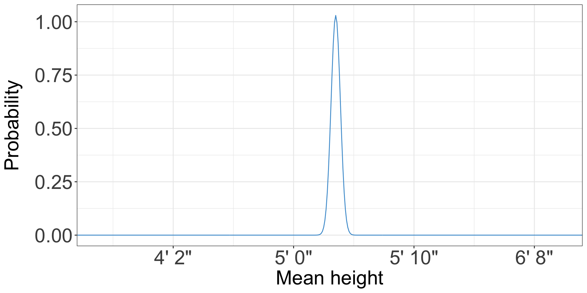
Sampling distributions

• Suppose you take a simple random sample of 100 women and find that they have a mean height of 5’ 4”
• You might take another sample, and find a mean height of 5’ 3”, or 5’ 5”
• The sampling distribution is the distribution of these means

Sampling distributions

The Central Limit Theorem

• The Central Limit Theorem is basically what makes statistics work
• It states that as samples get larger, statistics from those samples get closer to the corresponding parameters from the population

The Central Limit Theorem in real life

• Airline flight overbooking
• Grocery store stocking
• Power demand
• Traffic

The Central Limit Theorem

The sampling distribution of the mean of a simple random sample of \(n\) individuals has:

• Mean equal to the population mean
• Standard deviation equal to the population standard deviation divided by \(\sqrt{n}\)
  • This is called the standard error

• Note that this does not depend on the population size!
• So a 50-person sample is just as representative of a 500-person population as a 350 million person population
  • Assuming the sample is random
  • When the sample size starts to get close to the population size, the standard error is smaller than population standard deviation divided by \(\sqrt n\)
  • This is almost never the case in planning

Testing the Central Limit Theorem in Excel

• Let’s simulate sampling the height of women many times
• Open up Excel and enter =NORM.INV(RAND(), 63.5, 2.74) in cell A1
• This generates a random number drawn from a normal distribution with mean 63.5 and standard deviation 2.74
  • Equivalent to taking the height of a random American woman
• Fill this formula down the first 100 cells

Testing the Central Limit Theorem in Excel

• Let’s confirm that we got what we expected
• In cell A102, enter =AVERAGE(A1:A100)
• Since we generated random numbers from a distribution with mean 63.5, the average should be about 63.5
  • Not exactly, due to sampling error - it will come from the sampling distribution for the mean

Testing the Central Limit Theorem in Excel

• In cell A103, enter =STDEV(A1:A100)
• The standard deviation should be about 2.74

Testing the Central Limit Theorem in Excel

• Select cells A1 through A100
• Under the Insert tab, select the histogram icon, and insert a histogram
• It should look roughly like the distribution of women’s height we’ve seen so far

Testing the Central Limit Theorem in Excel

• We’ve simulated a single sample of 100 women
• Now we want to simulate many samples of 100 women
• Select cells A1 through A103, and drag them to the right to fill many columns
• Now we have many samples of 100, and means of each

Testing the Central Limit Theorem in Excel

• The mean of each sample comes from the sampling distribution for the mean
• We have many means from many samples of size 100
• What should the mean of the means be? 63.5
• What should the standard error of the means be? \(2.74 / \sqrt{100}\) = 0.274

Testing the Central Limit Theorem in Excel

• Compute the mean and standard deviation of the means
• Do you get approximately 63.5 and 0.274?

The Central Limit Theorem

• If the sample size is large, the sampling distribution of the mean is normal!
  • Regardless of whether the data are normal or not

• What is large? Some people say 35, some say 50, some say 100
• The further from normal your data is, the bigger the sample needs to be

Why did that have an exclamation point?

• Since the sampling distribution is normal, all the properties of the normal distribution above apply
• We can use those properties to quantify the accuracy of our estimates

Confidence intervals

• A confidence interval is a range and a probability
• For instance, a 90% confidence interval for the mean travel time to work in Chapel Hill is 18.7–20.5
• The interpretation of this is that, based on the sample size of the survey, there is a 90% probability that the actual mean commute time is in this range

Margins of error

• In the news media, margins of error are more common than confidence intervals
• The mean commute time in Chapel Hill is 19.6 minutes ± 0.9 minutes, with an 90% confidence
• This is equivalent, although the media often leaves out the confidence level

How do we know how far off we are if we don’t know the right answer?

• By applying the Central Limit Theorem!
• If we have a large sample, we know the sampling distribution of the sample mean is normal
• And that the mean of the sampling distribution is the population mean
• That means there’s a 95% chance that any given sample mean is within 1.96 standard errors of the population mean

How do we know how far off we are if we don’t know the right answer?

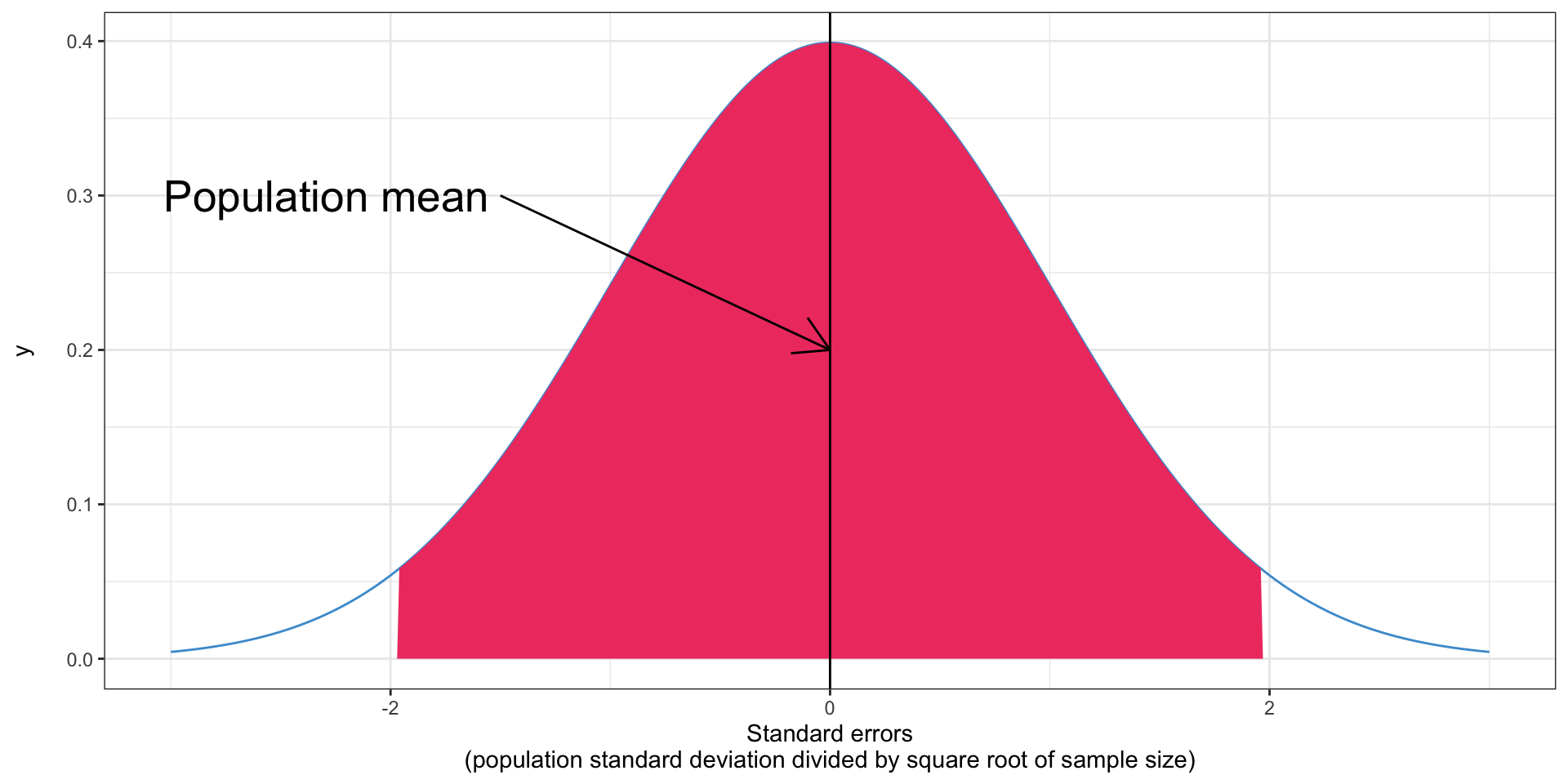
95% chance the sample mean is in the shaded area

But we don’t know the population mean!

• What do we know?
• We know the sample mean
• We know it’s within 1.96 standard errors of the population mean, with 95% confidence
• So the confidence interval is the sample mean plus and minus 1.96 times the standard error

Calculating a confidence interval

• Suppose we have taken a random sample of 100 US women and found an average height of 64 inches (5’ 4”)
• We know that the population standard deviation is 2.74 inches
• Let’s calculate the confidence interval for the population mean

Calculating a confidence interval

• First, calculate the standard error based on the population standard deviation (2.74) and the sample size (100): 0.274
• Multiply that by 1.96: .537
  • This is the 95% margin of error
• Add and subtract from the mean (64) to create the confidence interval: 63.473, 64.537
  • Does this include the population mean (63.5)?

Calculating a confidence interval

• Let’s calculate a 95% confidence interval for the height of US men
• We have sampled 81 men, and found an average height of 69.1 inches (5’ 9.1”)
• We know the population standard deviation is 2.25
• What is a 95% confidence interval for the mean?

Calculating a confidence interval

• Standard error of the mean: \(\frac{2.25}{\sqrt{81}} = 0.25\)
• Multiply by 1.96: 0.49
• Confidence interval: 68.61–69.59

What is special about 1.96?

• In a normal distribution, the center 95% is within 1.96 standard deviations of the mean
• You can confirm this in Excel if you want

What if we don’t know the standard deviation?

• In the examples above, I gave you the population standard deviation
  • This never happens in real life
• Instead, we have to approximate it with the sample standard deviation
• But this introduces additional error, so the confidence intervals should get bigger

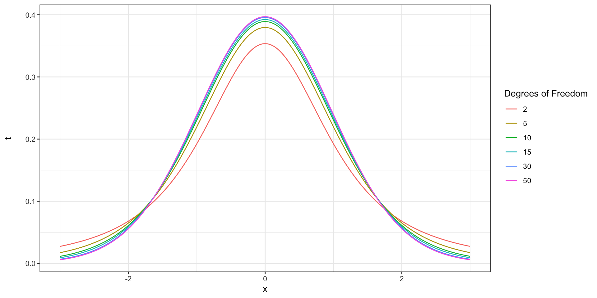
The \(t\) distribution

• The \(t\) distribution is very similar to the normal distribution, but with fat tails

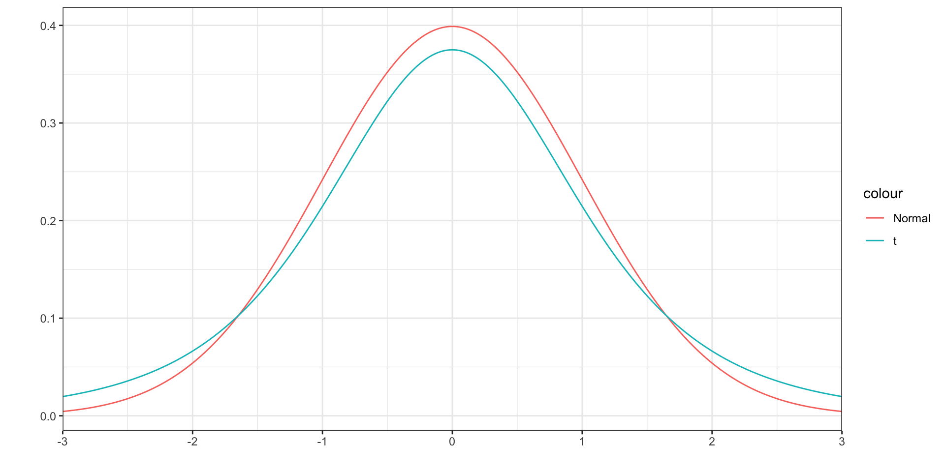
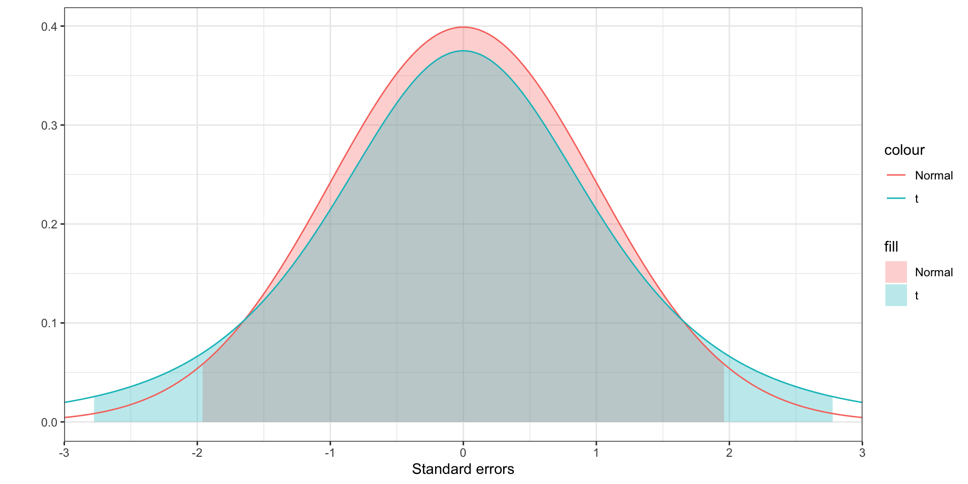
The \(t\) distribution

• This means that the center 95% is more spread out
• Instead of multiplying by 1.96, you’ll multiply by some larger number

Degrees of freedom

• The \(t\) distribution has a number associated with it called degrees of freedom
• This number is a measure of the sample size, and thus indirectly a measure of the quality of your estimate of the standard deviation
• The higher your sample size, the closer your sample standard deviation is likely to be to the population standard deviation
• The degrees of freedom you use in constructing a confidence interval is your sample size minus 1

Degrees of freedom

• The more degrees of freedom, the closer the \(t\) distribution is to the normal

Using the \(t\) distribution

• The only change is that instead of multiplying by 1.96, we multiply by a value determined by a \(t\) distribution (Washington, Karlaftis, and Mannering 2011)
• We want to find how many standard deviations from the mean contain 95% of the \(t\) distribution
• Unfortunately, this isn’t just a number we can remember, since it depends on the degrees of freedom
• This is called the critical value

Using the \(t\) distribution

• For a 95% confidence interval, the critical value is how many standard deviations below the mean the 2.5th percentile is
  • Or how many above the 97.5th percentile is
• 95% of the distribution is between the 2.5th and 97.5th percentiles
• You can look this up in a table of \(t\) critical values
• Or calculate it with Excel

Finding the critical value in Excel

• Use the T.INV function
• =T.INV(0.975, df) where df is degrees of freedom
  • 0.975 is the 97.5th percentile

Applying the \(t\) distribution

• Let’s use our 100-person sample of women again, but we don’t know the population standard deviation
• The sample mean is 64 inches
• The sample standard deviation is 2.75 inches
• Find the number of degrees of freedom (\(n-1\)): 99
• Find the critical value for a 95% confidence interval (use Excel): 1.98
• Find the standard error for the mean of a 100-person sample: \(2.75 / \sqrt{100}\) = 0.275
• Compute the margin of error by multiplying critical value and standard error: 0.55
• Calculate the confidence interval: 63.45–64.55

Applying the \(t\) distribution

• Let’s use our 81 person sample of men again
• We have sampled 81 men, and found an average height of 69.1 inches (5’ 9.1”)
• The sample standard deviation is 2.03
• What is a 95% confidence interval for the mean?

Applying the \(t\) distribution

• Find the number of degrees of freedom: 80
• Find the critical value for a 95% confidence interval: 1.99
• Find the standard error for the mean: \(\frac{2.03}{\sqrt{81}}\) = 0.23
• Find the margin of error: \(0.23 \times 1.99 = 0.45\)
• Find the confidence interval: \(69.1 \pm 0.45 = 68.65-69.55\)

Other confidence intervals (90%, 98%, etc)

• For other confidence levels, you just change the inputs when calculating the critical \(t\) value

Calculating confidence intervals in Excel

• Open (or download) the income data from last class
• Let’s calculate a 95% confidence interval for the mean income in North Carolina

Calculating what we need for the confidence interval

• Mean income: =AVERAGE(A:A) 68,228.58
• Sample standard deviation: =STDEV(A:A) 68,882.57
• Sample size: =COUNT(A:A) 50
• Standard error: \(\frac{68,882.57}{\sqrt{50}}\) 9,741.47
• Critical \(t\)-value: =T.INV(0.975, 49) 2.01
• 95% margin of error: \(2.01 \times 9,741.47\) 19,576.21
• Confidence interval: 48,652.37–87,804.79

Confidence intervals for proportions

• If the value you are calculating is proportion, the math is slightly different, as the standard deviation is not very meaningful
• The \(t\) distribution is not needed here
• You need a reasonably large sample, where the number of positive and negative responses are both greater than five
• The standard error is \(\frac{\sqrt{\hat p(1-\hat p)}}{\sqrt{n}}\), where \(\hat p\) is the estimated proportion from your data (Washington, Karlaftis, and Mannering 2011)

Confidence intervals for proportions

• Suppose we sample 200 commuters in New York State, and find that 65% of them commute by car
• Let’s compute a 95% confidence interval
• Standard error: \(\frac{\sqrt{0.65 \times (1 - 0.65)}}{\sqrt{200}}\) 0.034
• Margin of error: \(1.96 \times 0.03\) 0.067
• Confidence interval: 58.3%–71.7%

Confidence intervals for proportions in Excel

• Download the pums.xlsx file from Canvas
• This file contains data from the 2019 Integrated Public Use Microdata Sample, a sample of actual Census responses
• 100 commuters each from Illinois and Massachusetts

Confidence intervals for proportions in Excel

• Let’s calculate the confidence interval for the proportion of commuters who drive to work in Illinois
• First, let’s find the number of commuters who drove: =COUNTIF(A2:A101, "Auto, truck, or van") 85
• Next, the total number of commuters: =COUNTA(A2:A101) 100
  • Be sure not to include the column header in B1!
• Next, the proportion =D1 / D2 (your cells may vary) 0.85
• Next the standard error =SQRT(D3 * (1 - D3)) / SQRT(D2) 0.04
• The margin of error =1.96 * D4 0.07
• The confidence interval =D2 - D5, =D2 + D5 0.78, 0.92

Confidence intervals for proportions in Excel: Massachusetts

• Let’s calculate the confidence interval for the proportion of commuters who drive to work in Massachusetts
• First, let’s find the number of commuters who drove: =COUNTIF(A2:A101, "Auto, truck, or van") 82
• Next, the total number of commuters: =COUNTA(A2:A101) 100
  • Be sure not to include the column header in B1!
• Next, the proportion =D1 / D2 (your cells may vary) 0.82
• Next the standard error =SQRT(D3 * (1 - D3)) / SQRT(D2) 0.04
• The margin of error =1.96 * D4 0.08
• The confidence interval =D2 - D5, =D2 + D5, 0.74, 0.9

Hypothesis testing

• Confidence intervals give us a range of possible outcomes for the population mean
• Sometimes, we want to do a formal hypothesis test of whether the mean is different from a certain value, or different from another group

Hypothesis testing

• In hypothesis testing, we formulate two hypotheses
• \(H_0\) or the null hypothesis: the mean is not different
• \(H_1\) or the alternative hypothesis: the mean is different

• The hypothesis test allows us to either reject the null hypothesis as inconsistent with the data, or fail to reject the null hypothesis
• You cannot accept the null hypothesis

Hypothesis testing and the scientific method

• In the scientific method, we make hypotheses and then test them
• This is the underlying idea behind a hypothesis test
• In its purest form, we make a few hypotheses, do all the work, and everything boils down to a few hypothesis tests at the end

Millions of dollars, one test

• Physicists theorized that antimatter was affected by gravity
  • but competing theories were that it was not, or that it was affected oppositely
• To test this, they put 100 atoms of antihydrogen in magnetic “trap,” then turned off the magnets
• 70% of the atoms fell out the bottom
• They did a hypothesis test to confirm that this was statistically different from the null hypothesis of no effect

Anderson et al. (2023)

Formulating our hypotheses

• We know that the mean travel time to work in the US is 25.6 minutes from the Census
• In a sample of 100 Vermont commuters, the mean commute time was 22.4 minutes, with a standard deviation of 12.9 minutes
• Is the mean travel time in Vermont less than 25.6 minutes?

Formulating our hypotheses

• Null hypothesis: the mean travel time to work in Vermont is greater than or equal to 25.6 minutes
• Alternative hypothesis: the mean travel time to work in Vermont is less than 25.6 minutes

\[ H_0: \mu_{VT} \geq 25.6 \]

\[ H_1: \mu_{VT} < 25.6 \]

Testing our hypotheses: the one-tailed, one-sample \(t\)-test

• We can calculate our \(t\)-test with the sampling distribution under the null hypothesis
• This is what the sampling distribution would be, if the null hypothesis were true
• We evaluate the probability of getting a mean value of 22.4 or lower if this were the true sampling distribution, i.e. if the null hypothesis were true
• If the probability is below some pre-determined threshold \(\alpha\), we reject the null hypothesis as inconsistent with our data, and conclude that the mean travel time to work in Vermont is less than 25.6 minutes
• If we do so, we refer to the test as being statistically significant

The one-tailed, one-sample \(t\)-test

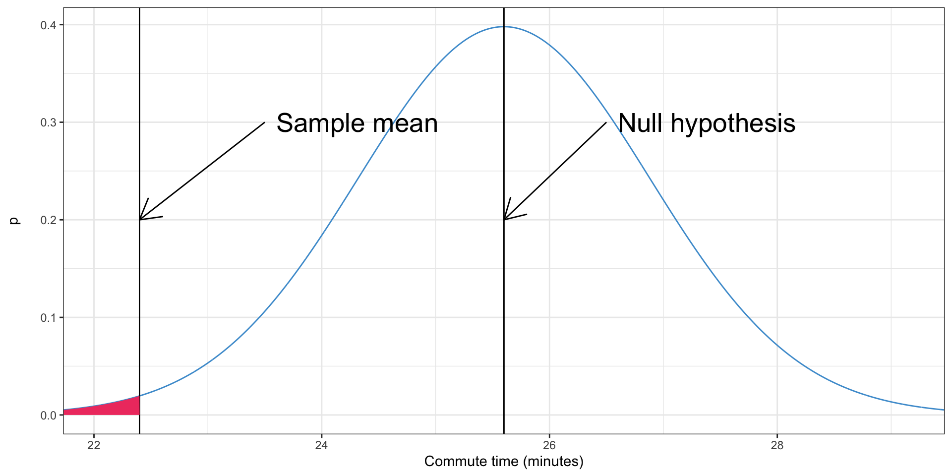
• The shaded area is a \(p\)-value

What is a \(p\)-value

• The probability of observing a sample mean more extreme than the one observed, if the null hypothesis were true
• If it is very unlikely, we reject the null hypothesis

Calculating the one-tailed, one-sample \(t\)-test in Excel

• First, we calculate the \(t\) test statistic, also known as the \(t\)-value
• In the case of the \(t\) test, this is the sample mean minus the value from the null hypothesis, divided by the standard error
• This is known as the \(t\)-value

\[ t = \frac{\bar x - x_0}{SE_{\bar x}} \]

• In this case, this is

\[ t = \frac{22.4 - 25.6}{12.9 / \sqrt{100}} = \frac{-3.2}{1.29} = -2.5 \]

Calculating the \(p\)-value from the \(t\)-value

• We need to use the \(t\) cumulative distribution function, just like we did for the normal distribution
• We need to find the degrees of freedom, which are just \(n-1\)
• Then we can calculate the \(p\)-value
• We can do this in Excel
• =T.DIST(t, df, TRUE)

Calculating the \(p\)-value from the \(t\)-value

• =T.DIST(-2.5, 99, TRUE) 0.007
• Based on this result, do we reject the null hypothesis, if \(\alpha = 0.05\)?
• What if \(\alpha = 0.01\)?

Calculating the one-tailed, one-sample \(t\)-test in Excel

• A recent Gallup poll found that Americans think a family of four needs to make $85,000/year to “get by”
• The mean income from the North Carolina income data we used previously was $68,228.58
  • Though this was not limited to families of four, and is several years old
• Based on this information, is the population mean less than $85,000?

Calculating the one-tailed, one-sample \(t\)-test in Excel

• Mean income: =AVERAGE(A2:A51), 68,229
• Standard deviation of income: =STDEV(A2:A51), 68,883
• Sample size: 50
• \(H_0\): \(\mu_{NC} \geq 85,000\)
• \(H_1\): \(\mu_{NC} < 85,000\)
• Standard error of the mean: \(\frac{68,883}{\sqrt{50}} = 9,741\)
• \(t\)-value: \(\frac{68,229 - 85,000}{9,741}\) = -1.72
• Degrees of freedom: 49
• \(p\)-value: =T.DIST(-1.72, 49, TRUE), 0.046
• Is it statistically significant at \(\alpha = 0.05\)? \(\alpha = 0.01\)?

What if we want to test if a value is greater than another?

• The MIT living wage calculator that a family of two adults needs to make $56,600 per year to get by in this region. Is the average NC wage at least larger than this?
• Mean income: =AVERAGE(A2:A51), 68,229
• Standard deviation of income: =STDEV(A2:A51), 68,883
• Sample size: 50
• \(H_0\): \(\mu_{NC} \leq 56,600\)
• \(H_1\): \(\mu_{NC} > 56,600\)
• Standard error of the mean: \(\frac{68,883}{\sqrt{50}} = 9,741\)
• \(t\)-value: \(\frac{68,229 - 56,600}{9,741}\) = 1.19
• Degrees of freedom: 49
• \(p\)-value: =T.DIST(1.19, 49, TRUE), 0.881

What if we want to test if a value is greater than another

• Which tail did we use? Which should we use?

What if we want to test if a value is greater than another?

• \(p\)-value: =1 - T.DIST(1.19, 49, TRUE), 0.119
• Is it statistically significant at \(\alpha = 0.05\)? \(\alpha = 0.01\)?

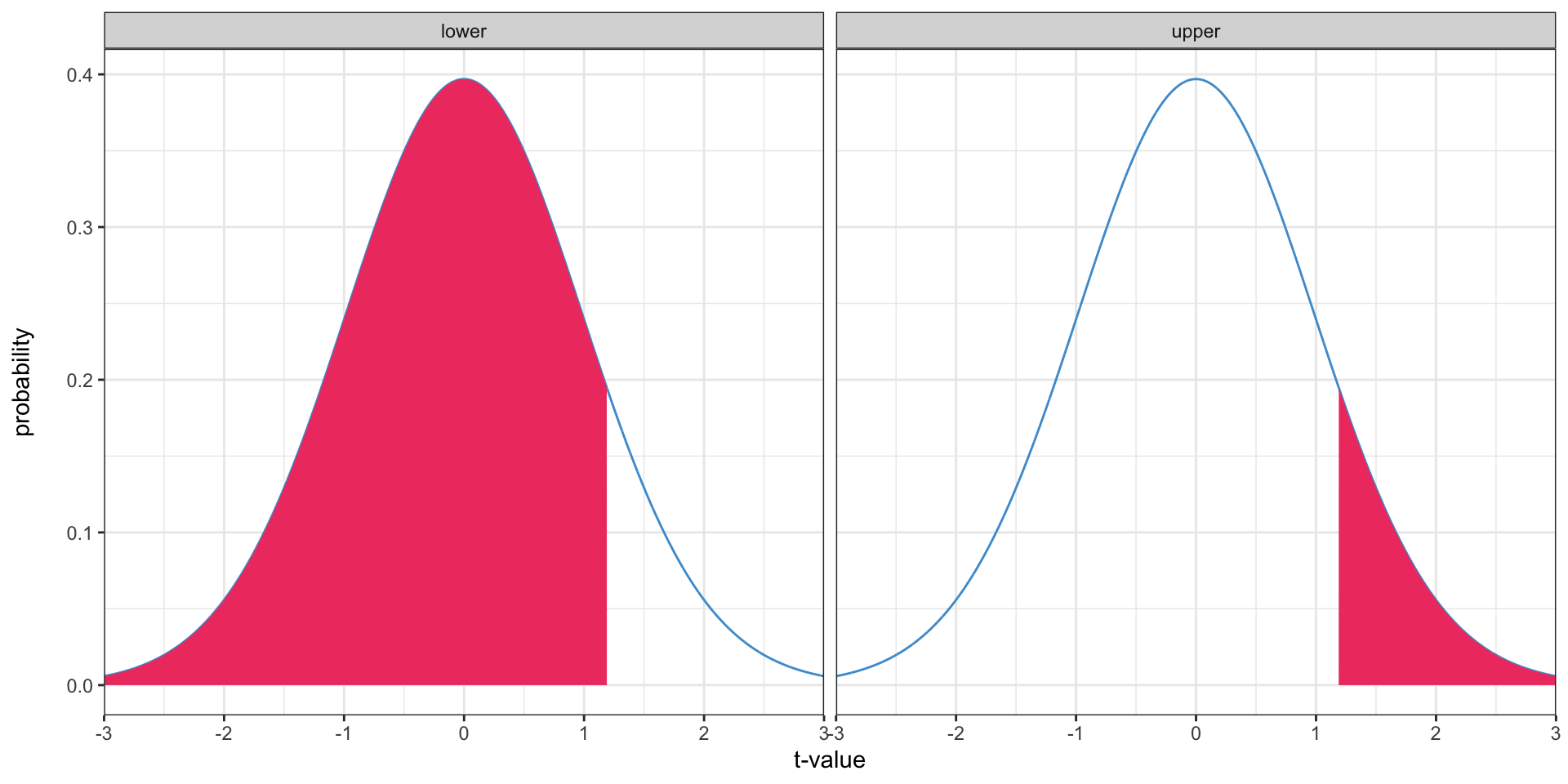
One-tailed tests

• Everything we’ve done so far has been a one-tailed test
  • Because we only used one tail of the distribution
• These are used to test whether one value is greater than another

© Walt Disney, source

Two-tailed tests

• Oftentimes, we won’t know beforehand whether the mean is greater than or less than the value we’re comparing it to, and only want to see if it’s different
  • We can’t just look at the sample mean to determine if it’s greater or less, because then we’re using some attribute of the sample mean to assume something about the population mean
  • This means we’re using information from the sample outside the test, so we’re not fully testing the sample
• The solution is a two-tailed test

Two-tailed tests

• What is the probability of getting a sample mean at least this far from the value in the null hypothesis?

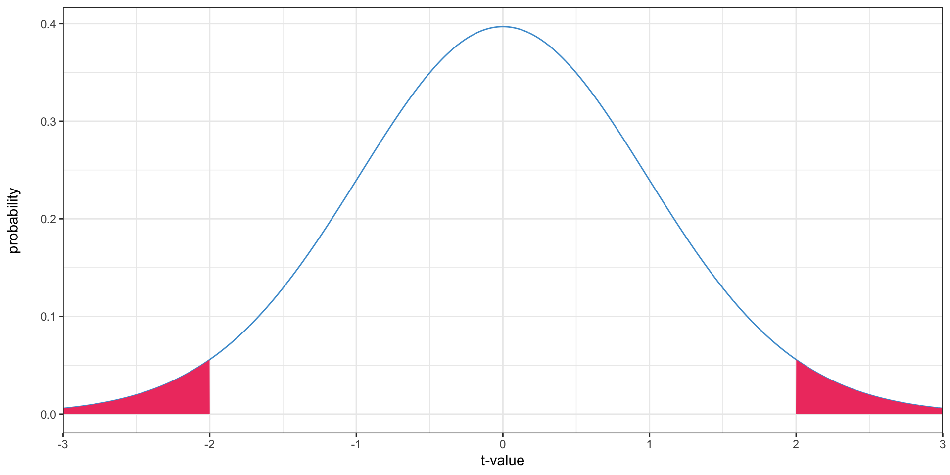
Two-tailed tests

• Since the \(t\) distribution is symmetrical, we can just double the \(p\)-value
• Excel also has the =T.DIST.2T() function for a two tailed test; all it does is double the probability value
• Two tailed tests are far more common than one-tailed tests

Calculating a two-tailed test

• Let’s once again use the North Carolina income data
• We know that Gallup has said that the living wage is $85,000/year, and we want to know whether the North Carolina mean income is higher or lower than this number

Calculating a two-tailed test

• Mean income: =AVERAGE(A2:A51), 68,229
• Standard deviation of income: =STDEV(A2:A51), 68,883
• Sample size: 50
• \(H_0\): \(\mu_{NC} = 85,000\)
• \(H_1\): \(\mu_{NC} \neq 85,000\)
• Standard error of the mean: \(\frac{68,883}{\sqrt{50}} = 9,741\)
• \(t\)-value: \(\frac{68,229 - 85,000}{9,741}\) = -1.72
• Degrees of freedom: 49
• \(p\)-value:
  • =T.DIST(-1.72, 49, TRUE) * 2, 0.091
  • =T.DIST.2T(1.72, 49), 0.091
• Can we conclude that the mean income in North Carolina is not $85,000, based on this sample?

Failing to reject vs. accepting

• When we fail to reject a null hypothesis, that does not mean that the null hypothesis is true or that the alternative hypothesis is false, only that given this data we cannot disprove the null hypothesis
• It could be that the null hypothesis is true,
• or it could be that we don’t have enough data to show that it is false

The relationship between confidence intervals and two-tailed tests

Video description

Animation showing the equivalence between confidence intervals and hypothesis tests. At the start, shows normal distribution centered on \(\bar x\), with the tails highlighted. The confidence interval is the range between the tails. The distribution then animates to the right to be centered on \(x_0\), with the tails still highlighted. One tail highlight starts at \(\bar x\) and the other starts an equal distance to the other side of \(x_0\). This demonstrates the equivalence of the two methods; the tails for the hypothesis test fall exactly at \(\bar x\), while a confidence interval with the same confidence level as the \(p\)-value of the hypothesis test has a tail that falls exactly at \(x_0\).

The relationship between confidence intervals and two-tailed tests

• When you construct a 95% confidence interval, you base it on the middle 95% of the sampling distribution
• When you perform a hypothesis test, it is statistically significant at the \(\alpha = 0.05\) level if less than 5% of the sampling distribution is further from the value in the null hypothesis than the sample mean
• If the confidence interval does not include the value in the null hypothesis, the hypothesis test will be significant, and vice-verse

Two-sample tests

• It’s often more useful to compare two samples to each other, rather than comparing a sample against a single value
• For instance, we might want to know whether commute times are different in urban vs rural areas, or traffic volumes are growing
• We don’t have a single value we are comparing against; both the means are from samples

Two-sample tests

• This is the test we want

\[ H_0: \mu_1 = \mu_2 \]

\[ H_1: \mu_1 \neq \mu_2 \]

Two-sample tests

• Two-sample tests work much the same way as one-sample tests
• We take the difference in means, and then use a one-sample test to see if that is different than zero
• We re-write this so we have a constant value we’re comparing against

\[ H_0 = \mu_1 - \mu_2 = 0 \]

\[ H_1 = \mu_1 - \mu_2 \neq 0 \]

The paired-sample \(t\)-test

• The paired-sample \(t\) test is the simplest two-sample \(t\)-test
• It is used when you have “paired” observations, often before-and-after
  • e.g. scores on a test, traffic volumes on roads before and after road diets
• The difference of the means is the mean of the differences
• So you can just take the difference from before to after,
  • average it,
  • and use a normal one-sample test

The paired-sample \(t\)-test

• Download the roadway_sensors.xlsx file from Canvas
• This has traffic volumes before and after the pandemic/lockdown at 196 randomly-selected sensors on California freeways, from a recent paper of mine
• We want to know if traffic volumes changed pre-pandemic to post-lockdown

The paired-sample \(t\)-test

• Create a new column with the difference in traffic flow pre-pandemic to post-lockdown: =B2-A2
• Do the normal \(t\)-test procedures with this column
• Mean: -4,179
• Standard deviation: 8,769
• Number of observations: 196
• Standard error: 626
• \(t\)-value: -6.67
• Degrees of freedom: 195
• \(p\)-value: \(2.6 \times 10^{-10}\)
• Are traffic volumes lower after the pandemic, at the \(\alpha = 0.05\) level?

Independent two-sample tests

• Suppose we have two samples, one from urban and one from rural areas (data from IPUMS)
  • The 144 urban respondents have a mean commute time of 23.6 min with a standard deviation of 16.2 min
  • The 100 rural respondents have a mean commute time of 21.0 min with a standard deviation of 17.5 min
• Do these two samples indicate that commute times are different in urban and rural areas?

Two-sample tests

• This works just like the paired test: we test that the difference is not zero
• \(H_0: \mu_{\mathrm{urban}} - \mu_{\mathrm{rural}} = 0\)
• \(H_1: \mu_{\mathrm{urban}} - \mu_{\mathrm{rural}} \neq 0\)
• The difference in means is 23.6 - 21.0 = 2.6 minutes
  • or 21.0 - 23.6 = -2.6 minutes, since this a two-tailed test you get the same answer either way
• Now we just apply the regular one-sample, two-tailed formula
• The standard error of this difference is uh, drat 🤔
• The degrees of freedom of the sampling distribution is oh, fiddlesticks 🤷

The sampling distribution of the difference in means

• Both means have a normal sampling distribution
• The difference of any two normal distributions is also normal
• Therefore, the sampling distribution of their difference is also normal
• This is a property of the normal distribution, but is not true of distributions in general

But wait, I thought the means had a \(t\) distribution?!

• The means are normally distributed, this is ensured by the Central Limit Theorem
• The problem is, we don’t know what the parameters of that normal distribution are (if we did, we wouldn’t need hypothesis tests)

Okay, so the difference of means is normally distributed. How does that help?

• We know it’s normally distributed
• But we still don’t know the standard error

The standard error of the difference in means

\[ SE(\bar x_1 - \bar x_2) = \sqrt{\frac{s_1^2}{n_1} + \frac{s_2^2}{n_2}} \]

where \(s_1\) is the standard deviation (not standard error) for the first sample, \(n_1\) is the sample size, likewise for \(s_2\) and \(n_2\)

source

Why?

• We can re-write that formula as

\[ SE(\bar x_1 - \bar x_2) = \sqrt{\left(\frac{s_1}{\sqrt{n_1}}\right)^2 + \left(\frac{s_2}{\sqrt{n_2}}\right)^2} \]

• You’ll recognize the parts in parentheses as the standard errors of the individual means
• So the standard error of the difference is something like the standard error of each one, summed up
  • With some squaring and square roots added

So we can again re-write as

\[ SE(\bar x_1 - \bar x_2) = \sqrt{SE(\bar x_1)^2 + SE(\bar x_2)^2} \]

Degrees of freedom of the difference in means

• We’re still basing this standard error on the sample standard deviations, so we still need the \(t\) distribution
• The degrees of freedom calculation is annoying

\[ \frac{ \left(\frac{s_1^2}{n_1} + \frac{s_2^2}{n_2}\right)^2 }{ \frac{\left(\frac{s_1^2}{n_1}\right)^2}{n_1-1} + \frac{\left(\frac{s_2^2}{n_2}\right)^2}{n_2 - 1} } \]

Excuse me what

• This is a ratio of powers of the standard error of the difference to the standard errors divided by the degrees of freedom of the individual means
• We can re-write that formula as

\[ \frac{ SE(\bar x_1 - \bar x_2)^4 }{ \frac{ SE(\bar x_1)^4 }{ df_1 } + \frac{ SE(\bar x_2)^4 }{ df_2 } } \]

where \(SE(\bar x_1)\) is the standard error of the mean of the first sample, \(SE(\bar x_1 - \bar x_2)\) is the standard error of the difference, and \(df_1\) is degrees of freedom for the mean of the first sample (with similar definitions for the second sample)

• I don’t have a good explanation for how the fourth powers get involved or why this is the exact formula
• This is called the Welch-Satterthwaite approximation if you’re looking for some bedtime reading
• If you’re doing this in the real world, use statistical software (e.g. R)

Back to our example

• Suppose we have two samples, one from urban and one from rural areas (data from IPUMS)
  • The 144 urban respondents have a mean commute time of 23.6 min with a standard deviation of 16.2 min
  • The 100 rural respondents have a mean commute time of 21.0 min with a standard deviation of 17.5 min
• The difference in means is 23.6 - 21.0 = 2.6 minutes

Standard error of the difference in means

\[ SE(\bar x_1 - \bar x_2) = \sqrt{\frac{s_1^2}{n_1} + \frac{s_2^2}{n_2}} \]

\[ \sqrt{\frac{16.2^2}{144} + \frac{17.5^2}{100}} = \]

2.21

Degrees of freedom calculation

• First, let’s calculate the standard errors and degrees of freedom for the two means separately
• Urban: \(\frac{16.2}{\sqrt{144}} =\) 1.35 , 143 degrees of freedom
• Rural: \(\frac{17.5}{\sqrt{100}} =\) 1.75 , 99 degrees of freedom
• Now, let’s calculate the degrees of freedom of the difference

\[ \frac{ SE(\bar x_1 - \bar x_2)^4 }{ \frac{ SE(\bar x_1)^4 }{ df_1 } + \frac{ SE(\bar x_2)^4 }{ df_2 } } \]

\[ \frac{ 2.21^4 }{ \frac{1.35^4}{143} + \frac{1.75^4}{99} } = \]

202.2 😅

Now, the test itself

• We have everything we need:
  • Difference in means: 2.6
  • Standard error of difference in means: 2.21
  • Degrees of freedom: 202.2
• \(t\)-value: \(\frac{2.6}{2.21} = 1.18\)
• \(p\)-value: =T.DIST.2T(1.18, 202.2) = 0.24
• Do we reject or fail to reject the null hypothesis that the means are the same?

The whole thing: let’s work through an example with real data

• Do people in North Carolina and South Carolina have different incomes?
• Go to the PUMS file we downloaded earlier
• There are sheets for North Carolina and South Carolina, that have income information

North and South Carolina incomes

• Calculate the means of income in the two states: NC: 87,610, SC: 91,286
• Calculate the standard deviations: NC: 84,232, SC: 81,782
• Calculate the difference in means: ±3,676
• Calculate the standard errors for the individual means: NC: 7,657, SC: 7,435
• Calculate the standard error for the difference: 10,673
• Calculate the degrees of freedom for the individual means: NC: 121, SC: 121
• Calculate the degrees of freedom for the whole thing: 239.8
• Calculate the (two-tailed) \(p\)-value: 0.73
• Is this statistically significant at the \(\alpha=0.05\) level? \(\alpha=0.01\)?

The equal-variance \(t\)-test

• The book also discusses an equal-variance \(t\)-test
• That’s a very strong assumption, especially if the means are not equal
• The unequal-variance test works ok when the variances are equal
• I would recommend against the equal-variance test
• More information in this paper

Hypothesis tests of categorical data: the \(\chi^2\) test

• Sometimes, you will want to test if two categorical outcomes are related
• For instance, is there a relationship between education and means of transportation to work in North Carolina?
• We can use a \(\chi^2\) (chi-squared) test for this

The cross-classification table

• The first step is to cross-classify the two variables
• The cross-classification table counts how many observations have each combination of the two variables

The cross-classification table

Education	Rural	Urban	Total
College	9	18	27
High school or some college	26	39	65
Less than high school	7	22	29
Total	42	79	121

• Is there any relationship between education and urbanity?
• It’s hard to tell, because there are more urban people in every category in this sample

The \(\chi^2\) test

• The \(\chi^2\) test compares the actual values in the cross-classification table with expected values assuming the null hypothesis of no relationship between the two variables
• The expected values are the row total multiplied by the column total divided by the overall total source

Why are these the expected values?

• This distributes the total for each row across the cells based on the relative values of all the columns
• The column total divided by the overall total is the proportion of all the observations in that column (e.g. the proportion urban)
• Multiplying by the row total distributes the values in the row according to the prevalence of each column
• Because multiplication is commutative, you can rearrange the formula to be the column total multiplied by the row total divided by the overall total, and the same logic applies

The \(\chi^2\) test statistic

• The \(\chi^2\) test statistic is the sum of the squared differences between observed and expected, divided by the expected values
• If \(O_{cr}\) is the observed count for column \(c\), row \(r\), \(E_{cr}\) is the expected count, and \(C\) and \(R\) are the number of columns and rows, then the test statistic is

\[ \chi^2 = \sum\limits_{c=1}^{C} \sum\limits_{r=1}^{R} \frac{\left(O_{cr} - E_{cr}\right)^2}{E_{cr}} \]

source

Properties of the \(\chi^2\) test statistic

• The \(\chi^2\) test statistic is a measure of how far the observed counts are from the expected
• Are the expected values always integers (whole numbers)?
• Is the test statistic ever negative?

How far is too far?

• You will basically never get observed counts that exactly match the expected
  • Especially since the expected counts are often non-integer
• Similar to how a sample mean never perfectly matches the population mean

The \(\chi^2\) test

• The \(\chi^2\) hypothesis test tests how likely we would be to observe a \(\chi^2\) value this large if the null hypothesis of no relationship were true
• If it is small (smaller than our chosen \(\alpha\)), then we reject the null hypothesis and conclude that there is a relationship between the two categories
  • We don’t know what the relationship is, just that it exists

The \(\chi^2\) distribution

• Because the \(\chi^2\) test statistic is always positive, it can’t be normal or \(t\)-distributed

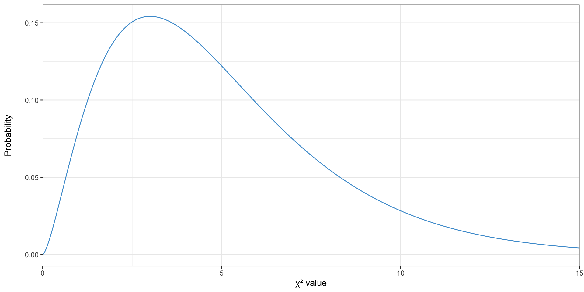
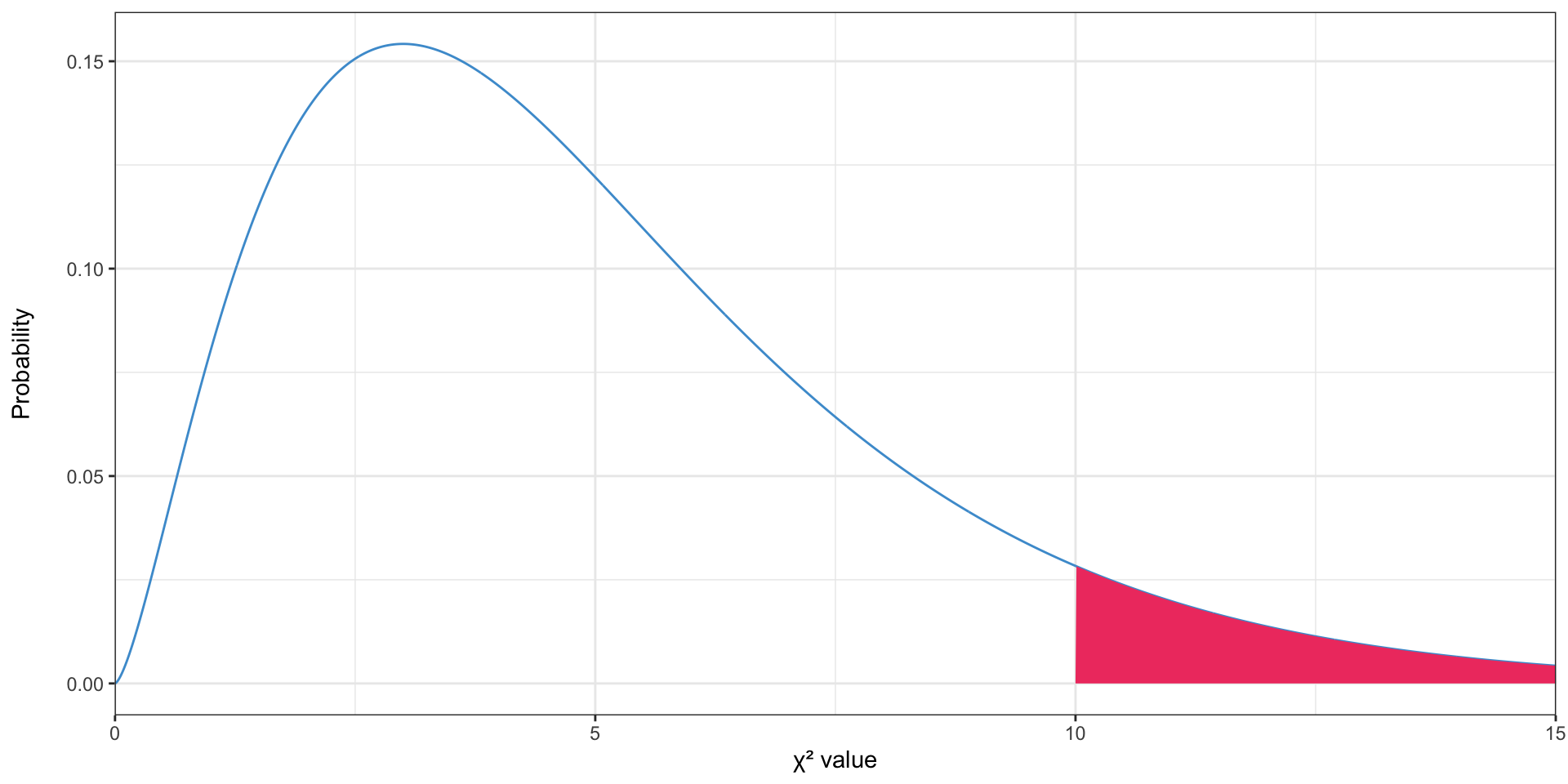
The \(\chi^2\) distribution

• The \(p\)-value is the area above the test statistic
• Like the \(t\) distribution, the \(\chi^2\) distribution has a degrees of freedom value, which is the number of rows minus one times the number of columns minus 1 (\((R - 1)(C - 1)\)) (source)

Why the \(\chi^2\) distribution? 😱

• The normal distribution kind of “makes sense” - it is symmetrical, values near the center are more likely
• The \(\chi^2\) distribution does not immediately make sense—it’s asymmetrical, how is the peak (mode) determined?

What are we doing in the \(\chi^2\) test? 😱

• We are taking the difference between the number of people in a category and the expected number of people in a category
• Let’s assume that both of these values are normally distributed
• Therefore the difference between them is normally distributed (with mean zero, under the null hypothesis)
• But then we square them - can they still be normally distributed?
  • Think about what \(2^2\) and \(-2^2\) are

Enter the \(\chi^2\) distribtuion 😱

• Conveniently, the \(\chi^2\) distribution is the distribution of a sum of squared standard normally distributed variables
• Which is exactly what we have

Sums of squares normally distributed values

Sums of squared values from 1000 samples of size 4 from a normal distribution

Compared to the \(\chi^2\) distribution with 4 degrees of freedom 😅

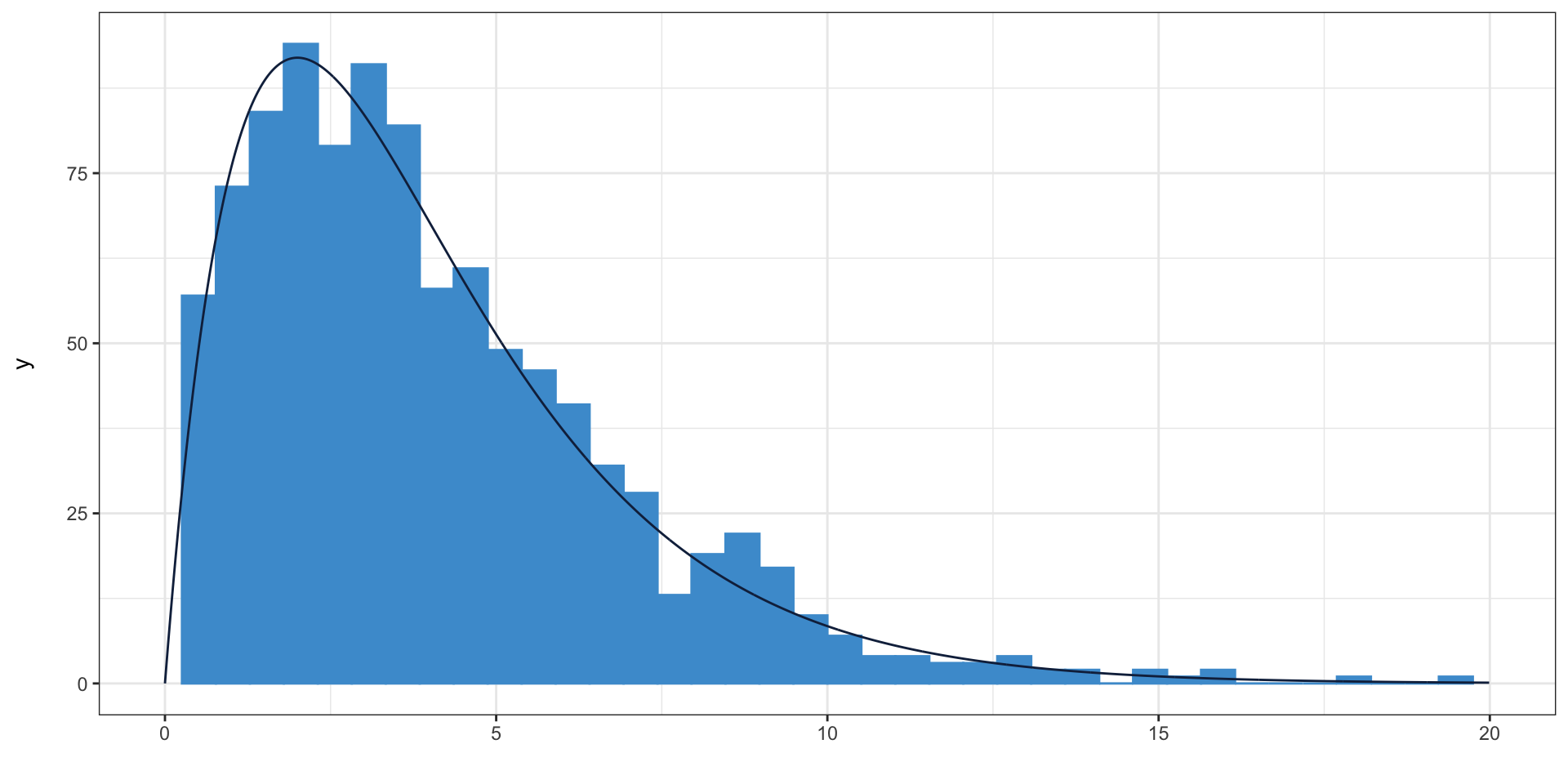
Sums of squared values from 1000 samples of size 4 from a normal distribution

Creating a cross-classification table in Excel

• To create a cross-classificaton table, we will use the PivotTable functionality in Excel
• Select the “Education” and “Urban/Rural” columns, and choose Insert PivotTable on the Insert toolbar
• Insert the PivotTable into the same sheet or into a new sheet
• Drag “Education” to rows and “Urban/Rural” to both Columns and Values; make sure that “Count of Urban/Rural” appears under values (source)

Creating a cross-classification table in Excel

Education	Rural	Urban	Total
College	9	18	27
High school or some college	26	39	65
Less than high school	7	22	29
Total	42	79	121

Calculating expected values in Excel

• The expected value is the row total multiplied by the column total, divided by the overall total
• The formula for this is relatively simple, e.g. =F5 * B8 / F8
• But we want to calculate expected values for all cells, not just one, and we don’t want to have to manually type the formula every time
• What happens if you expand this formula by dragging down or right?

Calculating expected values in Excel

• Preceding a column or a row label with $ will “lock” that label, so that expanding will not change it
  • $F$8 will always select F8, even when expanded
  • $F8 will always select column F, but the row number will change when expanded down
  • F$8 will always select row 8, but the column will change when expanded across

Calculating expected values in Excel

• How can we modify our formula to give correct expected values when expanded?

=F5 * B8 / F8

=$F5 * B$8 / $F$8

• Now, expand the formula to the right and down to calculate the rest of the expected values
• All of the expected values need to be at least five to use the \(\chi^2\) test (source)

Calculating expected values in Excel

Rural	Urban
9.37	17.63
22.56	42.44
10.07	18.93

Calculating the test statistic

• Now, we create cells with the squared difference between expected and observed, divided by the expected value
  • =(B5-B10)^2/B10
• And sum them up
  • =SUM(B13:D14)
• This is our test statistic: 2.255
• We have (3 - 1)(2 - 1) = 2 degrees of freedom
• Like the \(t\) distribution, we can use CHISQ.DIST to get the p-value
• We want the right tail, so we use the CHISQ.DIST.RT variant
• =CHISQ.DIST.RT(B18, 2): 0.324

Calculating the \(p\)-value

• There is also a CHISQ.TEST function
• You still need to calculate expected values by hand, but it will calculate the test statistic and calculate the \(p\)-value
• Then you just run =CHISQ.TEST(actual, expected) where actual and expected are cell ranges
  • e.g. =CHISQ.TEST(B5:D6, B13:D14)
• If you’re doing this a lot I would use statistical software, not Excel

Calculating the \(\chi^2\) test in Excel

• Are marital status and urban/rural status independent?

Cross-classification table

Marital Status	Rural	Urban	Total
Divorced	6	7	13
Married, spouse absent	1	0	1
Married, spouse present	16	30	46
Never married/single	16	39	55
Separated	2	1	3
Widowed	1	2	3
Total	42	79	121

Expected values

Rural	Urban
4.51	8.49
0.35	0.65
15.97	30.03
19.09	35.91
1.04	1.96
1.04	1.96

Results

• Test statistic: 4.753
• Degrees of freedom: 5
• \(p\)-value: 0.447

Don’t ever do this by hand

Use statistical software

t.test(ncdata$income, mu=85000) # One-sample, two-tailed t-test
t.test(sensors$time1 - sensors$time2) # Paired-sample t-test
t.test(ncdata$income, scdata$income, var.equal=F) # Two-sample t-test
chisq.test(data$educ, data$urbrur) # Chi-squared test

Average differences…

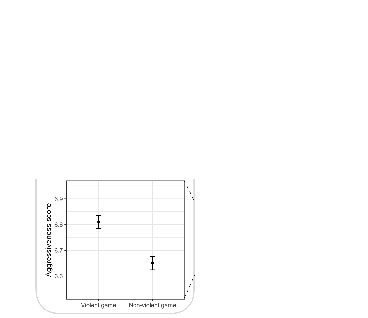
Zhang et al. (2022)

…do not translate to individual differences…

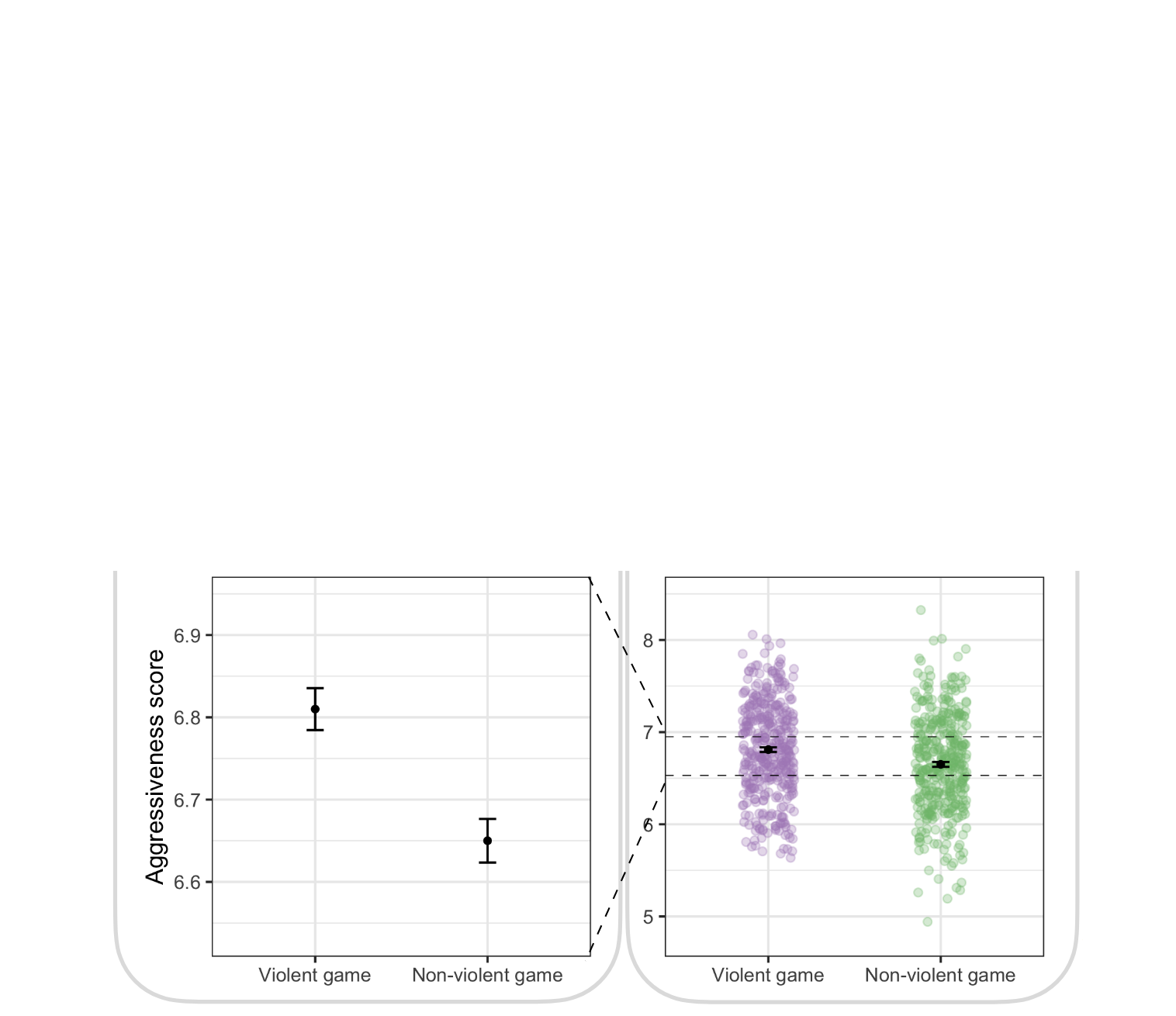
Zhang et al. (2022)

…and sample size matters

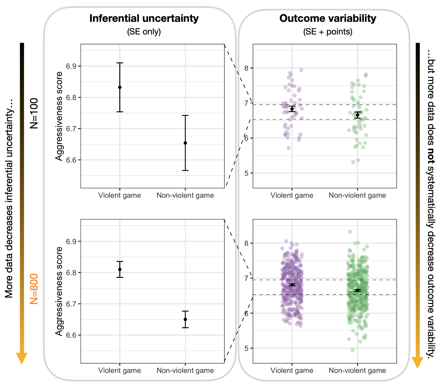
Zhang et al. (2022)

For next time

• Install R and RStudio

References

Anderson, E. K., C. J. Baker, W. Bertsche, N. M. Bhatt, G. Bonomi, A. Capra, I. Carli, et al. 2023. “Observation of the Effect of Gravity on the Motion of Antimatter.” Nature 621 (7980): 716–22. https://doi.org/10.1038/s41586-023-06527-1.

Arshad, Sidra, Shougeng Hu, and Badar Nadeem Ashraf. 2018. “Zipf’s Law and City Size Distribution: A Survey of the Literature and Future Research Agenda.” Physica A: Statistical Mechanics and Its Applications 492 (February): 75–92. https://doi.org/10.1016/j.physa.2017.10.005.

Washington, Simon, Matthew Karlaftis, and Fred Mannering. 2011. Statistical and Econometric Methods for Transportation Data Analysis. Boca Raton, FL: CRC Press.

Zhang, Sam, Patrick Ryan Heck, Michelle Meyer, Christopher F. Chabris, Daniel G. Goldstein, and Jake M. Hofman. 2022. “An Illusion of Predictability in Scientific Results.” SocArXiv. https://doi.org/10.31235/osf.io/5tcgs.

This work by Matthew Bhagat-Conway is licensed under a Creative Commons Attribution 4.0 International License.