| Person | Age | Personal Income | Density (persons/mi²) |
|---|---|---|---|
| 1 | 20 | 30,000 | 140,115 |
| 2 | 46 | 62,000 | 43,469 |
| 3 | 44 | 110,000 | 13,970 |
| 4 | 25 | 51,000 | 3,317 |
| 5 | 23 | 30,000 | 23,429 |
Regression
Matt Bhagat-Conway
Bivariate statistics
- So far, all the descriptive statistics we’ve dicussed have been univariate
- i.e. they described a single variable
- What if we instead wanted to describe the relationship between two variables?
The variance
- Remember that the variance is written out like this:
\[ Var(x) = \frac{\sum\limits_{i=1}^{n}(x_i - \bar x)^2}{n - 1} \]
Another way to write the variance
- We can also write this out like this:
\[ Var(x) = \frac{\sum\limits_{i=1}^{n}[(x_i - \bar x)(x_i - \bar x)]}{n - 1} \]
The covariance
- What if we want to introduce another variable and determine how they are related?
- e.g. income and age
- We can replace the second \(x_i - \bar x\) with an expression involving \(y\)
\[ Cov(x, y) = \frac{\sum\limits_{i=1}^{n}[(x_i - \bar x)(y_i - \bar y)]}{n - 1} \]
What does this do?
- Each observation of variable \(x\) is combined with the corresponding observation of variable \(y\)
- e.g. the income and age of the same person
- The deviations from the mean are multiplied together
- How does this measure the relationship between the variables?
The covariance, theoretically
- What is the sign of the product of the deviations?
| When x is… | |||
|---|---|---|---|
| Less than its mean | More than its mean | ||
| And y is… | Less than its mean | + | - |
| More than its mean | - | + | |
The outcome
- When both are above or below the mean, they contribute a positive value to the covariance
- When one is above and one is below, they contribute a negative value
Reasoning about covariance
- Do we expect a positive or negative covariance between age and income?
- What about between age and density?
Calculating covariance I
- Let’s calculate the covariance of age and income
| Person | Age | Personal Income | Density (persons/mi²) |
|---|---|---|---|
| 1 | 20 | 30,000 | 140,115 |
| 2 | 46 | 62,000 | 43,469 |
| 3 | 44 | 110,000 | 13,970 |
| 4 | 25 | 51,000 | 3,317 |
| 5 | 23 | 30,000 | 23,429 |
- Mean age: 31.6
- Mean income: 56,600
- Subtract the means from each value
Calculating covariance II
| Person | Age | Personal Income |
|---|---|---|
| 1 | −12 | −26,600 |
| 2 | 14 | 5,400 |
| 3 | 12 | 53,400 |
| 4 | −7 | −5,600 |
| 5 | −9 | −26,600 |
- Notice that the signs are always the same. Everyone with above-average age has above-average income and vice-versa
- What does this tell us about the covariance?
- Multiply the values together for each individual
Calculating covariance III
- Multiply the values together for each individual
| Person | Age | Personal Income | Product |
|---|---|---|---|
| 1 | −12 | −26,600 | 308,560 |
| 2 | 14 | 5,400 | 77,760 |
| 3 | 12 | 53,400 | 662,160 |
| 4 | −7 | −5,600 | 36,960 |
| 5 | −9 | −26,600 | 228,760 |
- Sum them up: 1,314,200
- Divide by \(n - 1\): 328,550
What does that mean?
- Like the variance, the covariance is in weird units
- Age deviation from mean is in years
- Income deviation from mean is in dollars
- Covariance is in dollar-years 🤔
The correlation coefficient
- We can’t just take the square root to get back to something reasonable
- Instead, we divide by the product of the standard deviations of the variables
- This gives us a value between -1 and 1
- -1: perfectly negatively correlated (when one goes up, the other goes down)
- 0: no relationship
- 1: perfectly positively correlated (when one goes up so does the other)
The correlation coefficient in math I
\[ Cor(x, y) = \frac{\quad\frac{\sum\limits_{i=1}^{n}[(x_i - \bar x)(y_i - \bar y)]}{n - 1}\quad}{s_x s_y} \]
The correlation coefficient in math II
- Rewrite with the full formula for standard deviation
\[ Cor(x, y) = \frac{\quad\frac{\sum\limits_{i=1}^{n}[(x_i - \bar x)(y_i - \bar y)]}{n - 1}\quad}{ \sqrt{\frac{\sum\limits_{i=i}^{n}(x_i - \bar x)^2}{n - 1}} \quad \sqrt{\frac{\sum\limits_{i=i}^{n}(y_i - \bar y)^2}{n - 1}} } \]
The correlation coefficient in math III
- Distribute the square roots in the standard deviations
\[ Cor(x, y) = \frac{\quad\frac{\sum\limits_{i=1}^{n}[(x_i - \bar x)(y_i - \bar y)]}{n - 1}\quad}{ \frac{\sqrt{\sum\limits_{i=i}^{n}(x_i - \bar x)^2}}{\sqrt{n - 1}} \quad \frac{\sqrt{\sum\limits_{i=i}^{n}(y_i - \bar y)^2}}{\sqrt{n - 1}} } \]
The correlation coefficient in math IV
- Multiply the numerators and denominators
\[ Cor(x, y) = \frac{\quad\frac{\sum\limits_{i=1}^{n}[(x_i - \bar x)(y_i - \bar y)]}{n - 1}\quad}{ \frac{ \sqrt{\sum\limits_{i=i}^{n}(x_i - \bar x)^2} \sqrt{\sum\limits_{i=i}^{n}(y_i - \bar y)^2} }{n - 1} } \]
The correlation coefficient in math V
- Cancel the \(n - 1\)
\[ Cor(x, y) = \frac{ \sum\limits_{i=1}^{n}[(x_i - \bar x)(y_i - \bar y)] }{ \sqrt{\sum\limits_{i=i}^{n}(x_i - \bar x)^2} \sqrt{\sum\limits_{i=i}^{n}(y_i - \bar y)^2} } \]
Calculating the correlation coefficient
- Multiply the values together for each individual
| Person | Age | Personal Income | Product |
|---|---|---|---|
| 1 | −12 | −26,600 | 308,560 |
| 2 | 14 | 5,400 | 77,760 |
| 3 | 12 | 53,400 | 662,160 |
| 4 | −7 | −5,600 | 36,960 |
| 5 | −9 | −26,600 | 228,760 |
- Sum them up: 1,314,200
- Square the age deviations from the mean and sum them up: 613
- Square the income deviations from the mean and sum them up: 4,327,200,000
- Take the square roots of the summed deviations: 24.76, 65,781
- Multiply the square roots together: 1,628,938
- Divide the summed products by the multiplied square roots: 0.81
What does the correlation coefficient mean
Calculating the correlation in Excel
- Excel has the
CORRELfunction to compute the correlation between two variables =CORREL(A:A, B:B)to calculate the correlation between income and age- Also calculate the correlations between age and density, and income and density
- Income and age: 0.2277803
- Age and density: 0.0719224
- Income and density: 0.1226299
Properties of the correlation coefficient
- Order doesn’t matter
- The correlation between age and income is the same as the correlation between income and age
- Location doesn’t matter
- Adding the same amount to everyone’s income won’t change the correlation
- Scale doesn’t matter
- If you expressed income in thousands of dollars, you would get the same correlation
\[ \frac{ \sum\limits_{i=1}^{n}[(x_i - \bar x)(y_i - \bar y)] }{ \sqrt{\sum\limits_{i=i}^{n}(x_i - \bar x)^2} \sqrt{\sum\limits_{i=i}^{n}(y_i - \bar y)^2} } \]
Moving beyond the correlation coefficient: simple linear regression
- The correlation coefficient tells us if there is a relationship, whether it is positive or negative, and how closely the two variables reflect each other
- It does not tell us anything about the scale of the relationship—i.e. how much change in one variable is associated with a one-unit change in the other?
- For this, we can use a linear regression
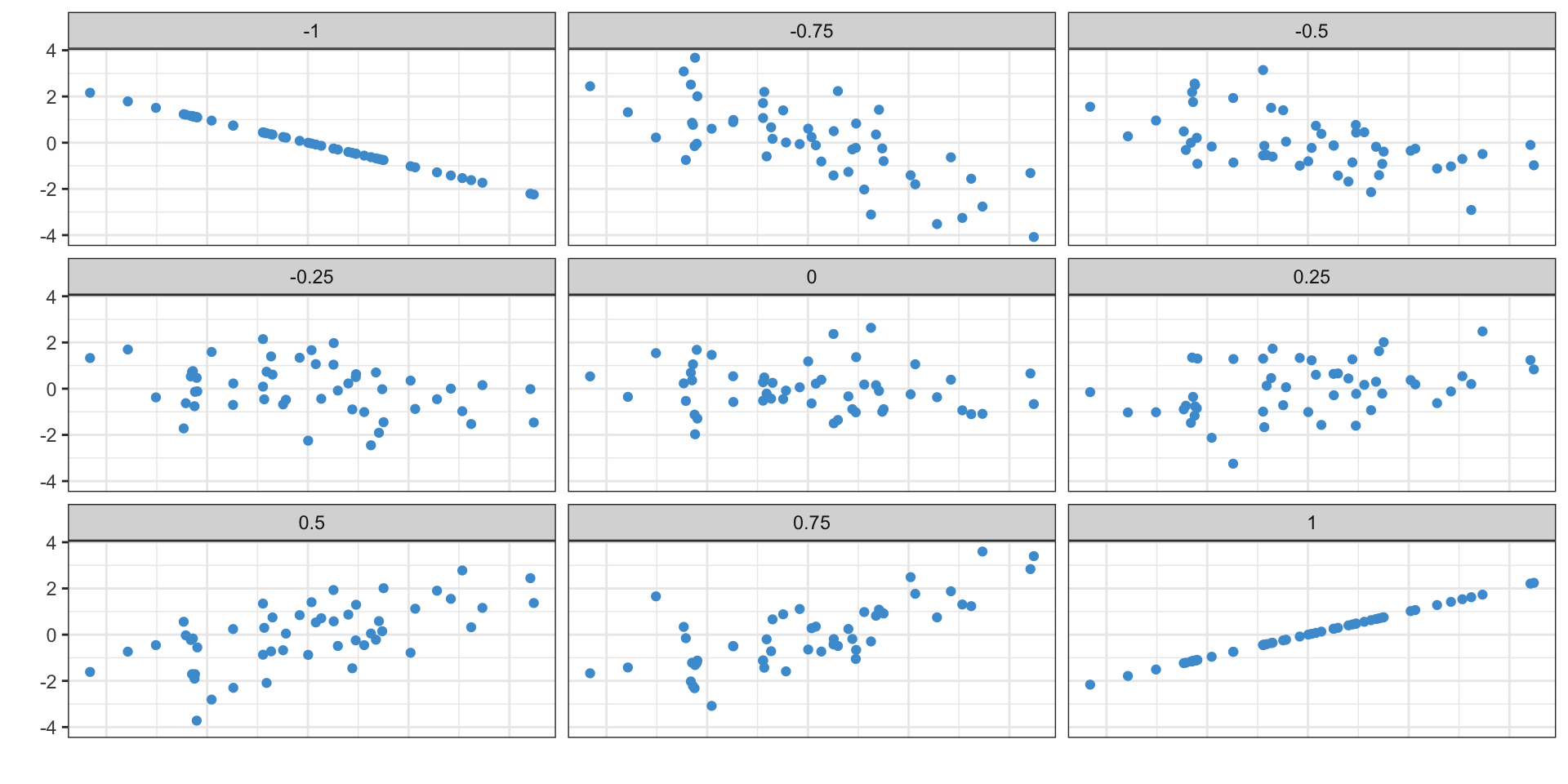
Simple linear regression
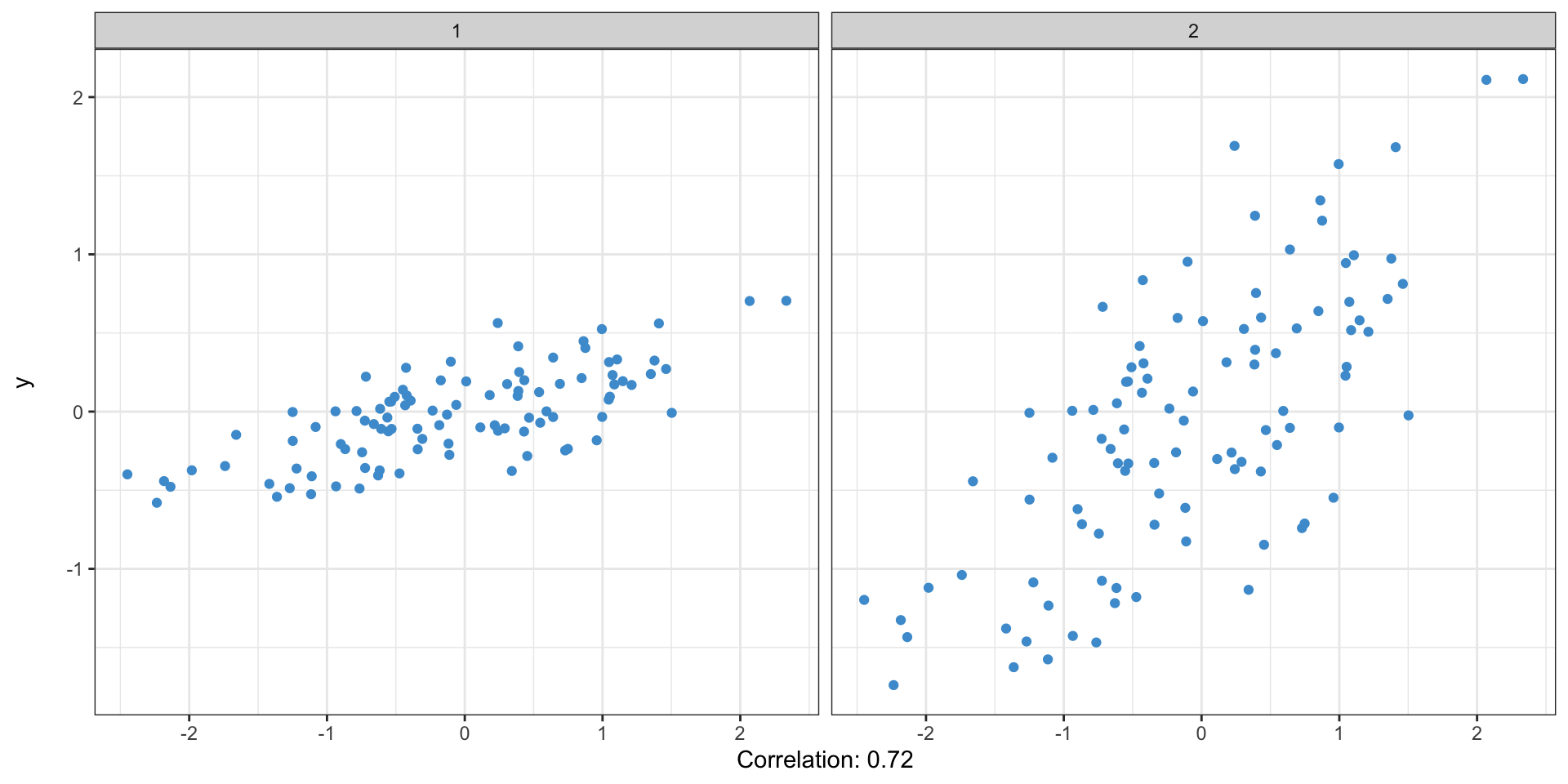
These both have the same correlation coefficient
Simple linear regression: interactive
\[ y = mx + b \]
\[ y = \alpha + \beta x \]
- \(y\) is also known as the dependent variable
- \(x\) is the independent variable
Simple linear regression: the idea
- In linear regression, we find the formula for the line that best “fits” the data
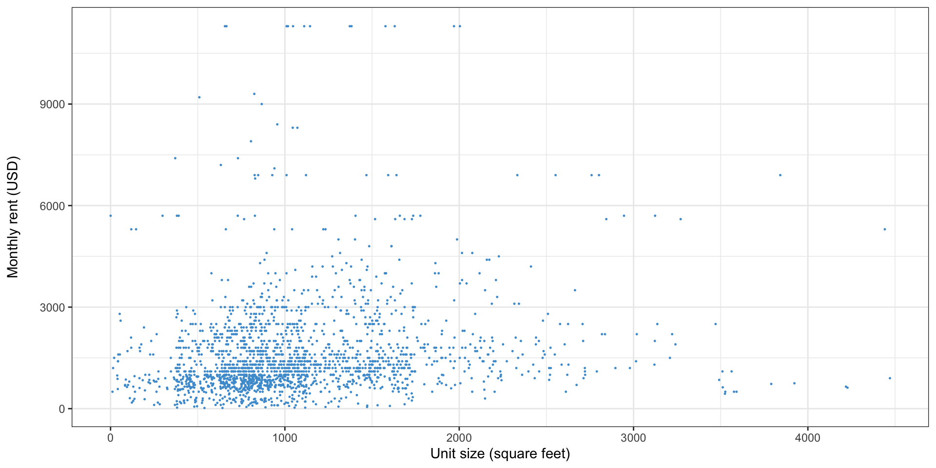
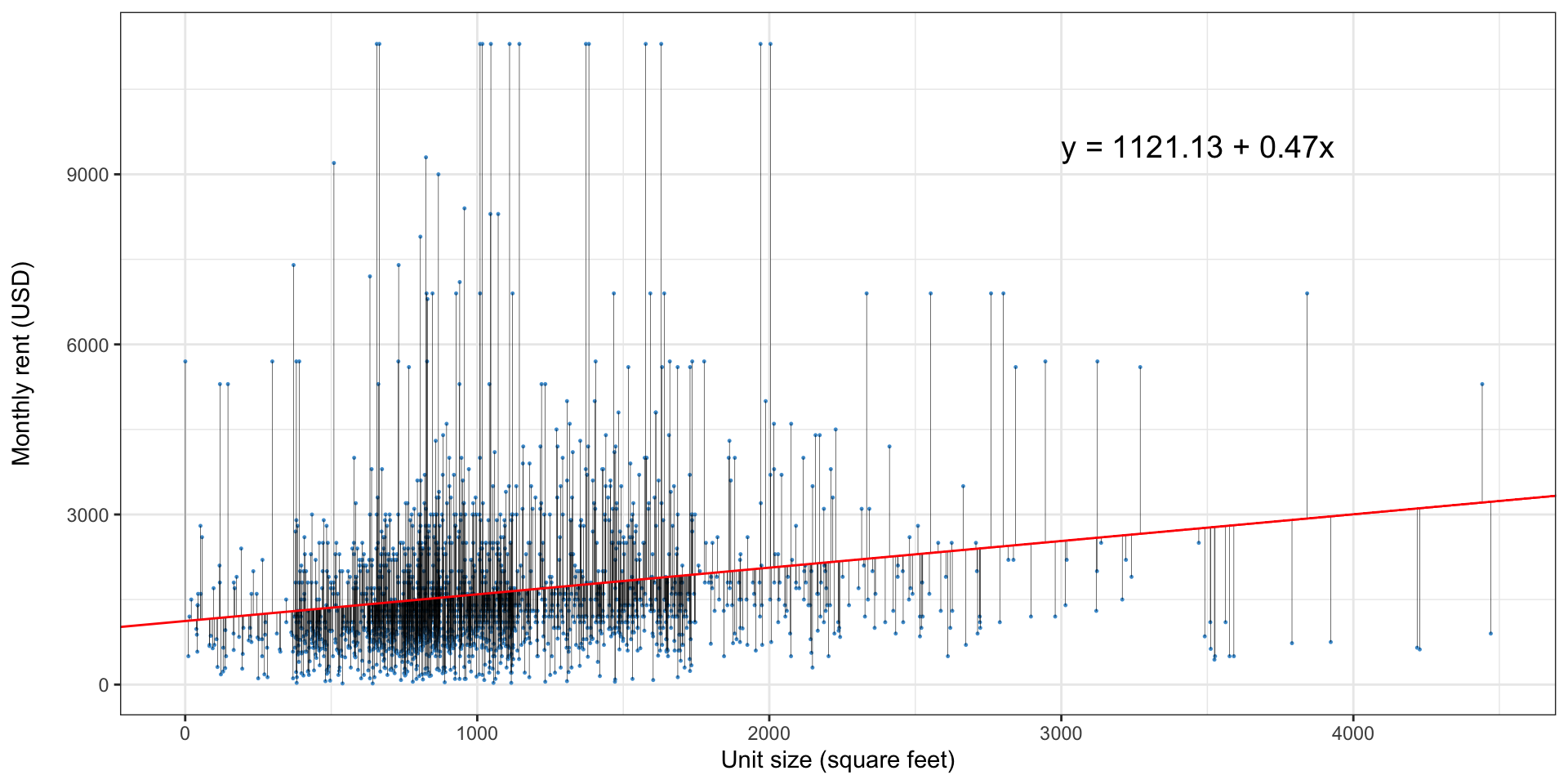
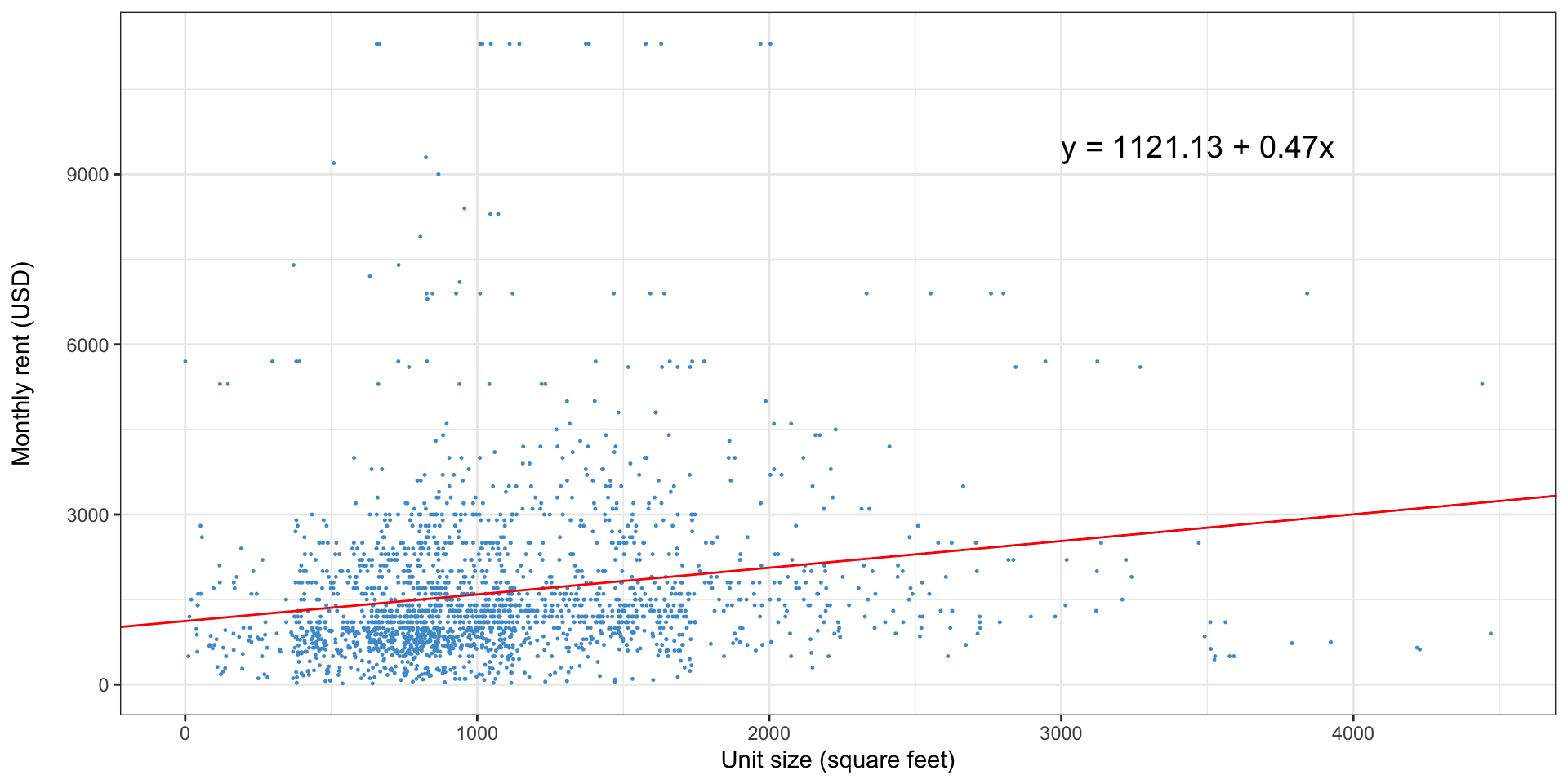
Simple linear regression: an example with data

- This graph shows unit size and monthly rent from the 2021 American Housing Survey1
- Do larger buildings have higher, lower, or the same rent?
- By how much?
Simple linear regression
Simple linear regression

Simple linear regression: how do we pick the line?

Simple linear regression: why not this line?
Simple linear regression: or this one?

What is a regression doing?
- Linear regression finds the line that minimizes the sum of squared residuals
- A residual is just the distance of each observation from the line
- For this reason, linear regression is sometimes called ordinary least squares or OLS
What is a regression doing, visually?
Where are the residuals in the regression formula
- We previously looked at the formula for a regression line:
\[ y = \alpha + \beta x \]
- This is the predicted value of y for a given value of x
- The full regression formula adds an error term which captures the residual
\[ y = \alpha + \beta x + \epsilon \]
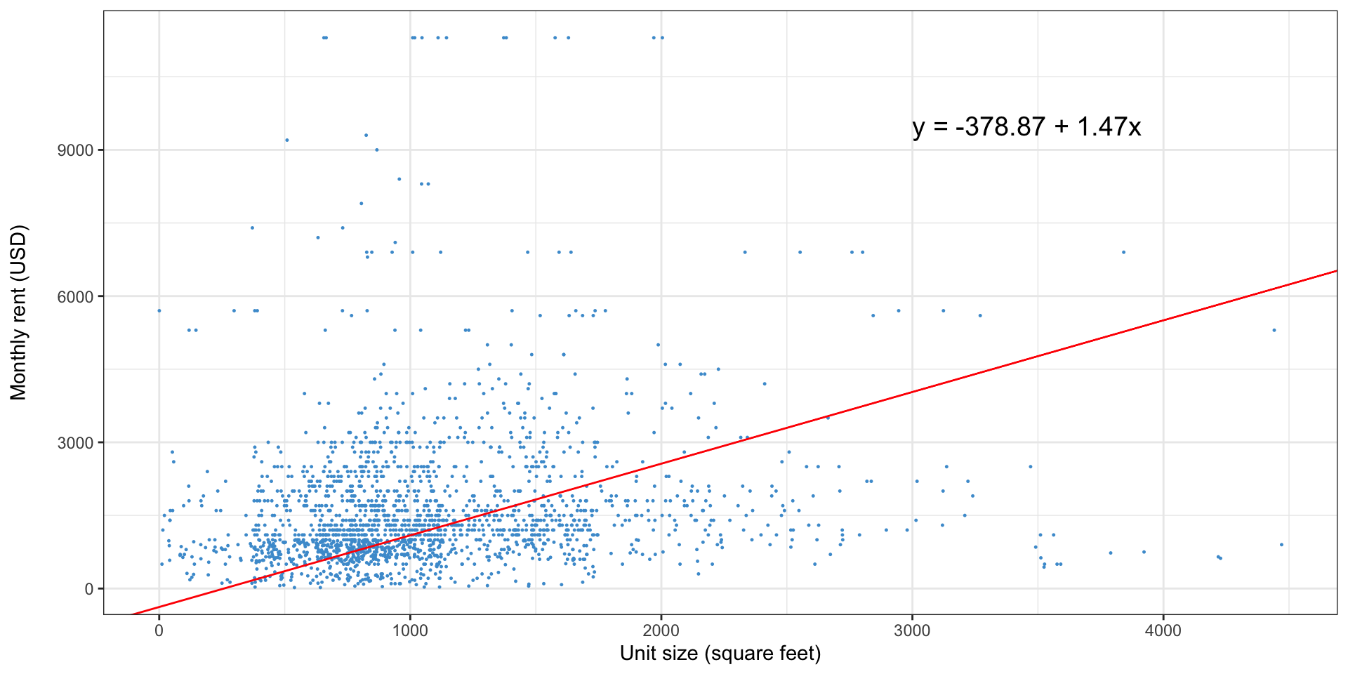
How do you interpret a regression?
- Are larger homes more expensive? Yes
- How much higher or lower would we expect the rent to be for a home that was 100 square feet larger? $47
- What does the intercept ($1,121) mean? The predicted price of a 0 sq ft. home
Reading a regression output
- Regressions are most often presented in tabular form
- Our regression of rent on building size would look like this
| Characteristic | Beta1 | SE | 95% CI | p-value |
|---|---|---|---|---|
| (Intercept) | 1,121*** | 71.7 | 981, 1,262 | <0.001 |
| UNITSIZE | 0.47*** | 0.059 | 0.36, 0.59 | <0.001 |
| R² | 0.031 | |||
| Adjusted R² | 0.031 | |||
| Statistic | 64.8 | |||
| p-value | <0.001 | |||
| No. Obs. | 2,000 | |||
| Residual df | 1,998 | |||
| Abbreviations: CI = Confidence Interval, SE = Standard Error | ||||
| 1 *p<0.05; **p<0.01; ***p<0.001 | ||||
Standard errors, \(p\)-values, and confidence intervals in regression
- Those last three columns probably sound familiar
- The SE column is the standard error of the coefficient estimate
- Like sample means, regression coefficients have a sampling distribution
- The regression output presents the standard errors (not deviations) for each coefficient
- Calculating these is nontrivial; let the software do it for you
- The sampling distribution is normal, but our standard error is estimated based on our sample, so we use the \(t\)-distribution
- The degrees of freedom are listed in “Residual df”, and are the sample size minus the number of coefficients (including the intercept)
Standard errors, \(p\)-values, and confidence intervals in regression
- The null hypothesis for the \(p\)-values is that the coefficient value is zero
- The interpretations are the same: the \(p\)-value is the probability of getting a regression coefficient this far from zero, if the true value were zero
- What does a regression coefficient of zero mean?
- Is this a one- or two-tailed test?
\(R^2\)
- The \(R^2\) is a measure of the goodness of fit of the regression
- Basically, how close is the regression line to the data?
- It ranges from 0 to 1, where 1 means it perfectly explains the data, and zero means it does not explain the data at all
- What a “good” \(R^2\) is depends on the context and what you’re trying to do
- e.g., regressions of human behavior have much lower \(R^2\) than something like house prices
- You can interpret it as the portion of the variance in the dependent variable that is explained by the independent variable
Prediction vs. interpretation
- There are two main uses for a regression
- In prediction, you use a regression to predict the \(y\) values for new \(x\) values
- In planning, for instance, this might be used to predict parking demand at a hotel being constructed
- In prediction, high \(R^2\) values are important to get precise predictions
Prediction vs. interpretation
- Interpretation is far more common in planning
- The regression coefficients are the finding, not predictions for some new set of \(x\) values
- For instance, we’re not trying to predict rents, we’re trying to understand what the relationship between home size and rents is
- For interpretation, high \(R^2\) is not as important
- Unless there are omitted variables—more on that soon
Linear regression in R
- Download the
AHS_2021.csvfile from Canvas - Open RStudio
- Create a new R script (File > New > R script)
- Save it to the same folder as the
AHS_2021.csvfile - Tell R to look in that directory: Session > Set Working Directory > To source file location
Linear regression in R
- R is a command-driven piece of software
- You interact with it by running text commands, rather than through a graphical interface
- An R script is just a file containing these commands, so that you can run them again at a later date, and keep track of what you’ve done
Linear regression in R
- We’re going to learn three commands:
read.csv,lm, andsummary - First, we need to load the data into R
- Anything after a
#character is ignored, I encourage you to use this “comment” functionality to take notes
Read data into R
View data in R
- You can see what R has read in by just typing
dataand pressing enter in the console - Or
View(data)to open up a spreadsheet-like viewer
Estimate a regression
- Let’s regress rent on number of bedrooms
- The
lmfunction estimates a regression - It takes two argument: the variables you want to use in your regression, and the data you want to use
Estimate a regression: code
- This will not print any output, but the result has been stored in the
modelvariable
Display a regression
The summary function will display regression results
Call:
lm(formula = RENT ~ BEDROOMS, data = data)

Residuals:
    Min      1Q  Median      3Q     Max
-2157.7  -774.7  -364.7   371.0  9671.0

Coefficients:
            Estimate Std. Error t value Pr(>|t|)
(Intercept)  1080.40      73.71  14.658   <2e-16 ***
BEDROOMS      274.32      32.72   8.385   <2e-16 ***
---
Signif. codes:  0 '***' 0.001 '**' 0.01 '*' 0.05 '.' 0.1 ' ' 1

Residual standard error: 1411 on 1998 degrees of freedom
Multiple R-squared:  0.03399,   Adjusted R-squared:  0.03351
F-statistic:  70.3 on 1 and 1998 DF,  p-value: < 2.2e-16
Interpreting regression results
- What is the relationship between number of bedrooms and rent?
- Is this statistically significant?
- What does it mean that it is statistically significant
- How much of the variance in rent is explained by number of bedrooms?
- Do the number of bedrooms alone do a good job of explaining rent?
Write out the regression equation based on the results
\(y=\) \(1080.4 +\) \(274.32x +\) \(\epsilon\)
Outliers
- Like means, regression is sensitive to outliers
- Because we square the residuals, high outliers will “pull” the regression line towards them
- How does our regression change if we remove any homes with rent over $5,000?
Regression without outliers
Call:
lm(formula = RENT ~ BEDROOMS, data = data[data$RENT <= 5000,
    ])

Residuals:
    Min      1Q  Median      3Q     Max
-1812.8  -591.7  -236.4   365.4  3363.6

Coefficients:
            Estimate Std. Error t value Pr(>|t|)
(Intercept)  1047.09      46.84  22.357   <2e-16 ***
BEDROOMS      196.43      20.95   9.378   <2e-16 ***
---
Signif. codes:  0 '***' 0.001 '**' 0.01 '*' 0.05 '.' 0.1 ' ' 1

Residual standard error: 878 on 1933 degrees of freedom
Multiple R-squared:  0.04351,   Adjusted R-squared:  0.04302
F-statistic: 87.94 on 1 and 1933 DF,  p-value: < 2.2e-16
How did removing these 65 homes change the results?
- Coefficient for bedrooms is much lower
- \(R^2\) is a bit better
Do we think that just one factor can explain rent?
- We’ve tried number of bedrooms and size of home
- Do we think there’s any single factor that explains how much rent is?
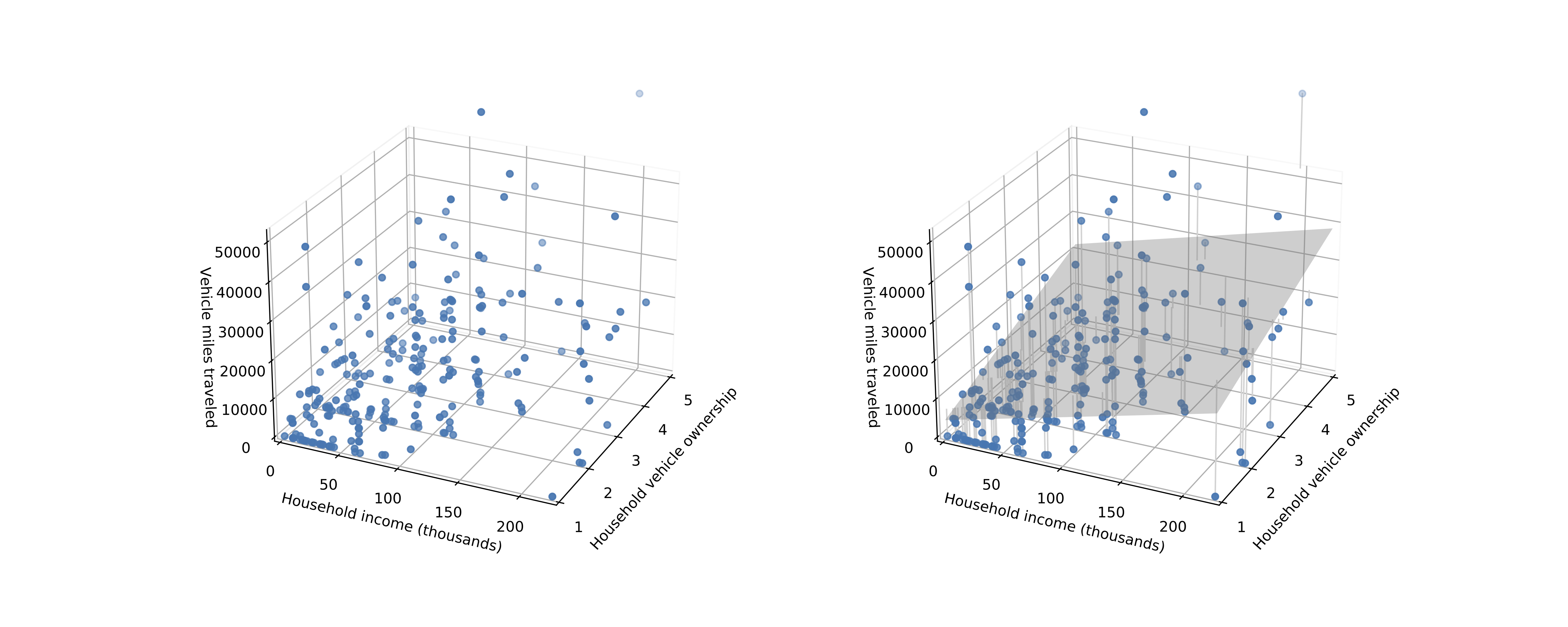
Multiple linear regression
- Simple linear regression can only evaluate the relationship between one variable and another
- Multiple linear regression explains evaluates the relationship between two or more independent variables and one dependent variable
Multiple linear regression: visually
Multiple linear regression: output
| Characteristic | Beta1 | SE | 95% CI | p-value |
|---|---|---|---|---|
| (Intercept) | 993*** | 78.1 | 840, 1,146 | <0.001 |
| UNITSIZE | 0.26*** | 0.078 | 0.11, 0.41 | <0.001 |
| BEDROOMS | 177*** | 43.9 | 91, 263 | <0.001 |
| R² | 0.039 | |||
| Adjusted R² | 0.038 | |||
| Statistic | 40.8 | |||
| p-value | <0.001 | |||
| No. Obs. | 2,000 | |||
| Residual df | 1,997 | |||
| Abbreviations: CI = Confidence Interval, SE = Standard Error | ||||
| 1 *p<0.05; **p<0.01; ***p<0.001 | ||||
Multiple linear regression in R
- In R, multiple linear regression is as simple as adding additional variables to the right-hand side of your regression with a
+sign - Let’s run a regression on unit size and year built (
YRBUILT)
Call:
lm(formula = RENT ~ UNITSIZE + YRBUILT, data = data)

Residuals:
    Min      1Q  Median      3Q     Max
-2483.5  -736.4  -369.9   382.9  9886.7

Coefficients:
              Estimate Std. Error t value Pr(>|t|)
(Intercept) -9.116e+03  2.569e+03  -3.549 0.000395 ***
UNITSIZE     4.667e-01  5.835e-02   7.998 2.12e-15 ***
YRBUILT      5.190e+00  1.302e+00   3.987 6.93e-05 ***
---
Signif. codes:  0 '***' 0.001 '**' 0.01 '*' 0.05 '.' 0.1 ' ' 1

Residual standard error: 1407 on 1997 degrees of freedom
Multiple R-squared:  0.03905,   Adjusted R-squared:  0.03809
F-statistic: 40.58 on 2 and 1997 DF,  p-value: < 2.2e-16
Multiple linear regression in R: more variables
- You can have more than two variables - add the number of bedrooms to the previous model
Call:
lm(formula = RENT ~ UNITSIZE + YRBUILT + BEDROOMS, data = data)

Residuals:
    Min      1Q  Median      3Q     Max
-2142.8  -747.0  -376.3   408.8  9850.7

Coefficients:
              Estimate Std. Error t value Pr(>|t|)
(Intercept) -9.878e+03  2.564e+03  -3.853  0.00012 ***
UNITSIZE     2.420e-01  7.818e-02   3.096  0.00199 **
YRBUILT      5.508e+00  1.298e+00   4.243 2.31e-05 ***
BEDROOMS     1.879e+02  4.375e+01   4.294 1.84e-05 ***
---
Signif. codes:  0 '***' 0.001 '**' 0.01 '*' 0.05 '.' 0.1 ' ' 1

Residual standard error: 1401 on 1996 degrees of freedom
Multiple R-squared:  0.04785,   Adjusted R-squared:  0.04642
F-statistic: 33.43 on 3 and 1996 DF,  p-value: < 2.2e-16
Overfitting
- There are two \(R^2\) values presented
- We’ve already talked about the standard \(R^2\), called “multiple \(R^2\)” here
- The adjusted \(R^2\) adds a penalty based on the number of predictors relative to the sample size
- This is to account for overfitting
- Overfitting is when you throw so many variables into the model that the model can exploit random chance to predict really well (e.g. maybe it just so happens in this dataset that the number of letters in the street name is highly predictive of rent)
Categorical variables


- What is the difference between these homes?
Categorical variables


- Location, location, location!
Categorical variables
- Our AHS dataset has a variable
METRONAMEthat contains the metropolitan area the home is in - How do we include this in a regression?
Categorical variables
- Your first thought might be to just re-code the variable to numbers, e.g. 1=Minneapolis, 2=Richmond, 3=San José, 4=Tampa, etc.
- If we coded the variable this way and put it in our regression, what are we assuming about the relationship between prices in these cities?
- The average price in these cities comes in this order
- The differences between cities are all the same
- Are either of these likely to be true?
Dummy coding
- The most common solution is to create dummy variables
- You create one new variable for each category of your categorical variable
- That new variable is 1 if the observation is in that category, and 0 otherwise
- You then put all of these variables into your regression, except one (we’ll see why in a minute)
Dummy coding
| City | Minneapolis | Richmond | Tampa | Oklahoma City |
|---|---|---|---|---|
| Minneapolis | 1 | 0 | 0 | 0 |
| Richmond | 0 | 1 | 0 | 0 |
| Minneapolis | 1 | 0 | 0 | 0 |
| Tampa | 0 | 0 | 1 | 0 |
| Richmond | 0 | 1 | 0 | 0 |
| Oklahoma City | 0 | 0 | 0 | 1 |
Dummy coding
- Our regression equation now looks like this:
\[ y = \alpha + \beta_1 \mathrm{Minneapolis} + \beta_2 \mathrm{Richmond} + \beta_3 \mathrm{Tampa} + \beta_4 \mathrm{OklahomaCity} + \beta_6 \mathrm{Bedrooms} + \epsilon \]
- We can’t estimate this, we need to remove one of the cities (it doesn’t matter which one)
- Why?
- Will the estimates change if we added one to \(\alpha\) and subtracted one from \(\beta_1\)—\(\beta_4\)?
- There is no unique solution
- So we remove one city
- Effectively, we are constraining that cities effect to zero
- All the other cities’ \(\beta\mathrm{s}\) will be relative to the left-out or “base” city
- Which city you leave out affects how you interpret the model, but does not affect the model’s predictions or goodness of fit
Dummy coding in action
| Characteristic | Beta1 | SE | 95% CI | p-value |
|---|---|---|---|---|
| (Intercept) | 767*** | 92.6 | 586, 949 | <0.001 |
| METRONAME | ||||
| Minneapolis-St. Paul-Bloomington, MN-WI | — | — | — | |
| Oklahoma City, OK | 84 | 99.6 | -112, 279 | 0.4 |
| Richmond, VA | -107 | 103 | -309, 95 | 0.3 |
| San Jose-Sunnyvale-Santa Clara, CA | 1,050*** | 91.2 | 871, 1,229 | <0.001 |
| Tampa-St. Petersburg-Clearwater, FL | -148 | 101 | -346, 51 | 0.14 |
| BEDROOMS | 289*** | 30.8 | 229, 350 | <0.001 |
| R² | 0.157 | |||
| Adjusted R² | 0.155 | |||
| Statistic | 74.5 | |||
| p-value | <0.001 | |||
| No. Obs. | 2,000 | |||
| Residual df | 1,994 | |||
| Abbreviations: CI = Confidence Interval, SE = Standard Error | ||||
| 1 *p<0.05; **p<0.01; ***p<0.001 | ||||
Interpreting the model with dummy variables
- Our \(R^2\) is much higher - a lot of the variation in price is due to the location
- Among the city variables, only San José is statistically significant
- What does this mean? What is the null hypothesis?
- The null hypothesis is that San José rents are equal to rents in the base category—Minneapolis
- Additional bedrooms still add value
Using dummy variables in R
- If you include a textual variable in your regression specification, R will automatically treat it as categorical
- If you have a numeric variable that you want to treat as categorical, put
factor(variable)in the model - Add
METRONAMEandBLDTYPE(building type) to your R model, and run it again
Using dummy variables in R: code
Call:
lm(formula = RENT ~ BLDTYPE + METRONAME + UNITSIZE + BEDROOMS,
    data = data)

Residuals:
    Min      1Q  Median      3Q     Max
-3074.3  -534.5  -136.6   217.2  9969.9

Coefficients:
                                                   Estimate Std. Error t value
(Intercept)                                       644.24922   99.53834   6.472
BLDTYPESingle family                              -94.37313   79.75814  -1.183
BLDTYPETrailer, mobile home, boat, RV, van, etc. -646.81135  236.34569  -2.737
METRONAMEOklahoma City, OK                        105.45456  100.50465   1.049
METRONAMERichmond, VA                             -97.21605  102.68464  -0.947
METRONAMESan Jose-Sunnyvale-Santa Clara, CA      1057.07199   90.86762  11.633
METRONAMETampa-St. Petersburg-Clearwater, FL     -111.81644  101.59910  -1.101
UNITSIZE                                            0.26395    0.07389   3.572
BEDROOMS                                          221.90817   45.94583   4.830
                                                 Pr(>|t|)
(Intercept)                                      1.21e-10 ***
BLDTYPESingle family                             0.236855
BLDTYPETrailer, mobile home, boat, RV, van, etc. 0.006261 **
METRONAMEOklahoma City, OK                       0.294190
METRONAMERichmond, VA                            0.343884
METRONAMESan Jose-Sunnyvale-Santa Clara, CA       < 2e-16 ***
METRONAMETampa-St. Petersburg-Clearwater, FL     0.271219
UNITSIZE                                         0.000363 ***
BEDROOMS                                         1.47e-06 ***
---
Signif. codes:  0 '***' 0.001 '**' 0.01 '*' 0.05 '.' 0.1 ' ' 1

Residual standard error: 1313 on 1991 degrees of freedom
Multiple R-squared:  0.1663,    Adjusted R-squared:  0.163
F-statistic: 49.65 on 8 and 1991 DF,  p-value: < 2.2e-16
Interpreting regressions: control variables
- The interpretation of the coefficients is a little different in a multiple regression
- Each coefficient is the association between that independent variable and the dependent variable, holding all other variables constant
- For example, the relationship between home size and rent, holding number of bedrooms constant
- Coefficients often change when adding other variables to the model
- For instance, do we expect an additional square foot of home to be as valuable if the number of bedrooms is held constant?
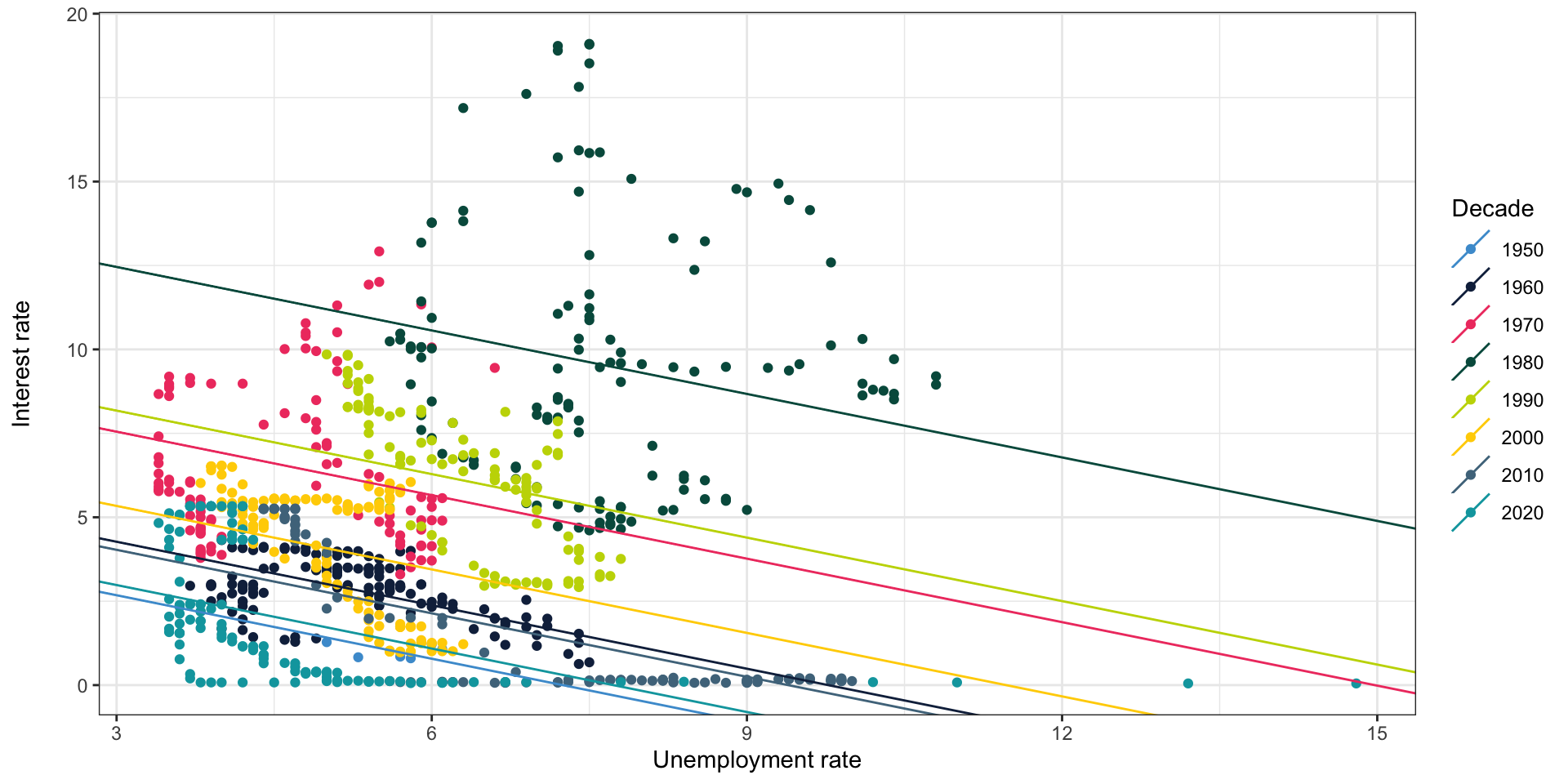
Simpson’s paradox
- In some cases, adding a control variable may even cause a coefficient to flip sign
- This is known as Simpson’s paradox
- This might happen, for instance, if homes in more expensive cities were smaller
- If you don’t control for city, smaller homes look more expensive—because those smaller homes are in more expensive locations
- When you do control for city, smaller homes look cheaper—holding city constant (i.e. within each city), smaller homes are cheaper
Simpson’s paradox
- We’re going to look at a plot of unemployment rate and federal interest rate
- Do we expect these to have a positive or negative correlation?
Simpson’s paradox: data
- Does it look like they have the expected relationship?
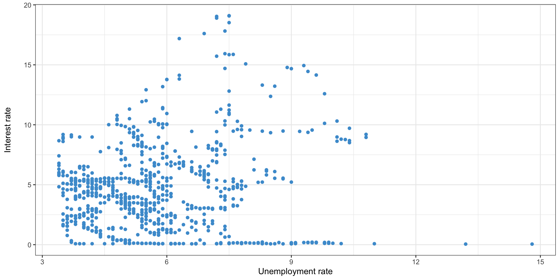
Adding the regression line
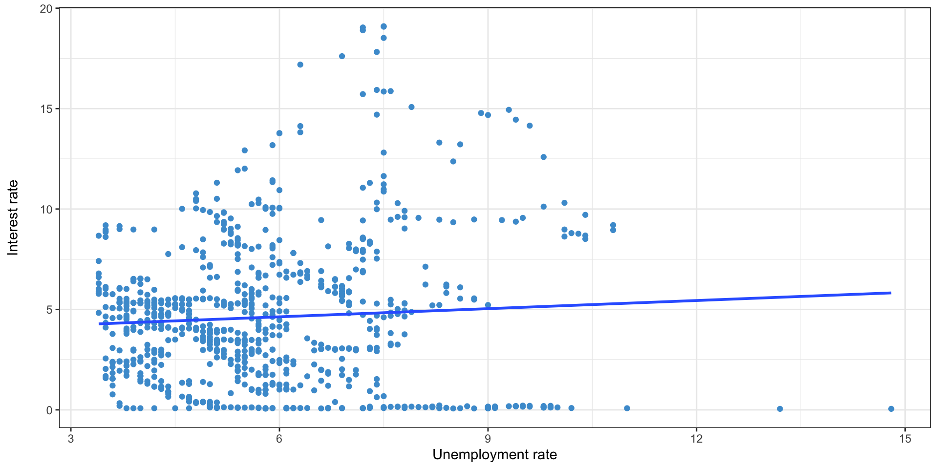
- y = 3.82 + 0x
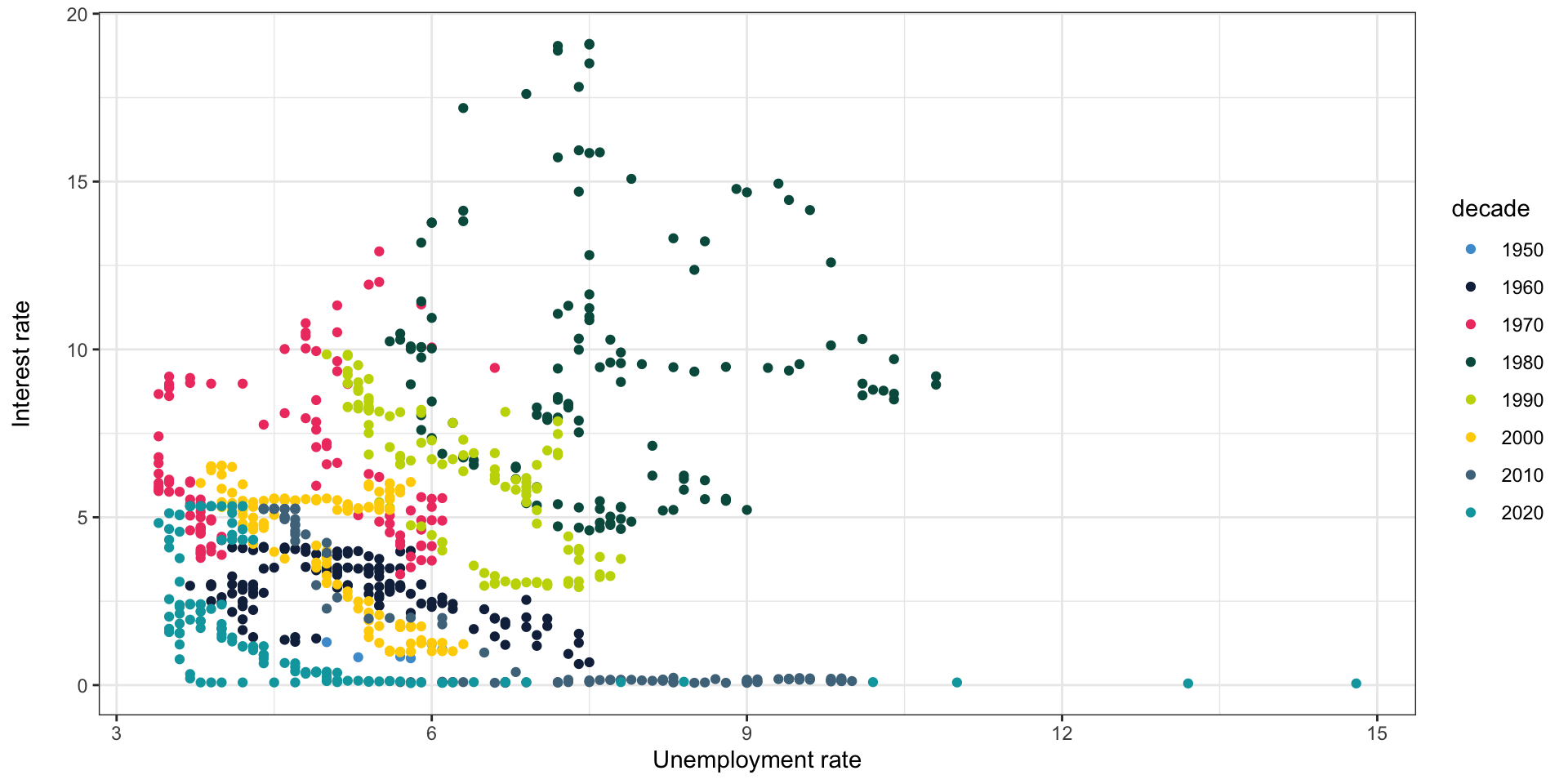
Adding another variable
- What if we control for decade?
Adding the regression lines
Interaction terms
- Used when we think the effect of one variable might vary based on the value of another
- Done by multiplying two variables together, and including them in the model as a new variable
- Most often done with dummy variables, as it is easier to interpret
- For instance, how does the cost of a bedroom vary by metro area?
Interaction terms
| Characteristic | Beta1 | SE | 95% CI | p-value |
|---|---|---|---|---|
| (Intercept) | 953*** | 152 | 654, 1,251 | <0.001 |
| METRONAME | ||||
| Minneapolis-St. Paul-Bloomington, MN-WI | — | — | — | |
| Oklahoma City, OK | -229 | 227 | -675, 216 | 0.3 |
| Richmond, VA | 102 | 237 | -364, 567 | 0.7 |
| San Jose-Sunnyvale-Santa Clara, CA | 609** | 193 | 230, 988 | 0.002 |
| Tampa-St. Petersburg-Clearwater, FL | -245 | 232 | -700, 211 | 0.3 |
| BEDROOMS | 189** | 72.4 | 47, 331 | 0.009 |
| METRONAME * BEDROOMS | ||||
| Oklahoma City, OK * BEDROOMS | 163 | 105 | -43, 368 | 0.12 |
| Richmond, VA * BEDROOMS | -86 | 107 | -296, 125 | 0.4 |
| San Jose-Sunnyvale-Santa Clara, CA * BEDROOMS | 228* | 89.7 | 52, 404 | 0.011 |
| Tampa-St. Petersburg-Clearwater, FL * BEDROOMS | 60 | 104 | -144, 263 | 0.6 |
| R² | 0.163 | |||
| Adjusted R² | 0.160 | |||
| Statistic | 43.2 | |||
| p-value | <0.001 | |||
| No. Obs. | 2,000 | |||
| Residual df | 1,990 | |||
| Abbreviations: CI = Confidence Interval, SE = Standard Error | ||||
| 1 *p<0.05; **p<0.01; ***p<0.001 | ||||
Interpreting interaction terms
- As with any dummy variable, we have a left-out category; the un-interacted bedrooms coefficient measures the cost in this city (Minneapolis)
- The interaction term is the difference from the base effect
- For instance, a bedroom in San José is worth $228 more than a bedroom in Minneapolis
- The \(p\)-value measures the statistical significance of the difference in effects
- We can concludes that bedrooms in San José are worth more than Minneapolis, and the difference is statistically significant
Interaction terms in R
- Just add a
*instead of a+between variables - For instance,
model = lm(RENT ~ METROAREA * BEDROOMS, data)includes and interaction between metro area and bedrooms
Collinearity
- What will happen if we add total rooms in addition to bedrooms to the model?
Collinearity
- Without total rooms
| Characteristic | Beta1 | SE | 95% CI | p-value |
|---|---|---|---|---|
| (Intercept) | 679*** | 95.5 | 492, 867 | <0.001 |
| BEDROOMS | 190*** | 41.1 | 110, 271 | <0.001 |
| UNITSIZE | 0.26*** | 0.073 | 0.12, 0.41 | <0.001 |
| METRONAME | ||||
| Minneapolis-St. Paul-Bloomington, MN-WI | — | — | — | |
| Oklahoma City, OK | 80 | 99.3 | -114, 275 | 0.4 |
| Richmond, VA | -111 | 103 | -312, 90 | 0.3 |
| San Jose-Sunnyvale-Santa Clara, CA | 1,049*** | 90.9 | 871, 1,227 | <0.001 |
| Tampa-St. Petersburg-Clearwater, FL | -149 | 101 | -347, 49 | 0.14 |
| R² | 0.163 | |||
| Adjusted R² | 0.160 | |||
| Abbreviations: CI = Confidence Interval, SE = Standard Error | ||||
| 1 *p<0.05; **p<0.01; ***p<0.001 | ||||
- With total rooms
| Characteristic | Beta1 | SE | 95% CI | p-value |
|---|---|---|---|---|
| (Intercept) | 400** | 128 | 149, 651 | 0.002 |
| BEDROOMS | 13 | 68.1 | -121, 146 | 0.9 |
| UNITSIZE | 0.20** | 0.076 | 0.05, 0.35 | 0.008 |
| METRONAME | ||||
| Minneapolis-St. Paul-Bloomington, MN-WI | — | — | — | |
| Oklahoma City, OK | 63 | 99.2 | -132, 257 | 0.5 |
| Richmond, VA | -108 | 102 | -309, 93 | 0.3 |
| San Jose-Sunnyvale-Santa Clara, CA | 1,067*** | 90.8 | 889, 1,245 | <0.001 |
| Tampa-St. Petersburg-Clearwater, FL | -135 | 101 | -332, 63 | 0.2 |
| TOTROOMS | 159** | 48.7 | 64, 254 | 0.001 |
| R² | 0.167 | |||
| Adjusted R² | 0.164 | |||
| Abbreviations: CI = Confidence Interval, SE = Standard Error | ||||
| 1 *p<0.05; **p<0.01; ***p<0.001 | ||||
Collinearity
- Bedrooms are no longer significant
- Why?
- Bedrooms and total rooms are highly correlated (correlation 0.89)
- The regression has a hard time differentiating them
- If we were to take a new sample, small differences might cause large changes in how rent is divided among bedrooms and total rooms
- The standard errors get much larger
Assumptions of linear regression
- The relationship is linear (can be addressed through variable transformations, e.g. squaring or logarithms)
- The observations (specifically, the error terms) are independent (only affects standard errors; can be addressed through clustering adjustments to standard errors)
- The errors have the same standard deviation regardless of predicted value (only affects standard errors; can be addressed through heteroskedasticity adjustments to standard errors)
Multiple testing
- When running a regression, you’re doing a lot of hypothesis tests (one per coefficient)
- Remember that a statistically significant hypothesis test means that there is a low probability that you would find this coefficient if there were truly no relationship between the variables
Multiple testing
| 0.1 | -0.09 | -0.17 | -0.03 | 0.07 | -0.12 | 0.07 | 0 |
| 0.09 | -0.03 | -0.06 | -0.02 | -0.06 | -0.15 | -0.13 | -0.08 |
| 0.08 | 0.16 | 0.22 | -0.17 | 0.01 | 0.05 | 0.23 | -0.2 |
| -0.04 | -0.11 | -0.19 | -0.2 | -0.16 | -0.05 | 0.01 | -0.27* |
| 0.02 | 0.09 | -0.06 | -0.01 | 0.22 | -0.01 | 0.12 | 0.19 |
(* = p < 0.05, ** = p < 0.01, *** = p < 0.001)
Multiple testing
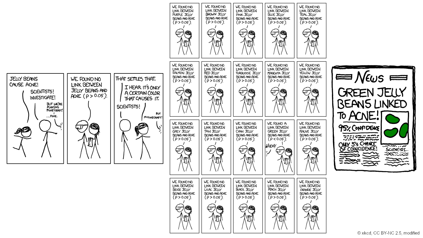
© xkcd
Multiple testing
- Best defense: use theoretically justified variables, don’t just try everything
\(p\)-hacking
- \(p\)-hacking is when someone tries many models, or many forms of model, in hopes of eventually getting a \(p\)-value below 0.05 for some variable of interest
- This is bad, because it means that the result of your research is pre-determined; the research itself is meaningless
- This can also happen through the publication process
- If 20 teams are working on a problem, and one finds statistically significant results, that may be the only result that gets published

This work by Matthew Bhagat-Conway is licensed under a Creative Commons Attribution 4.0 International License.
Footnotes
the unit size variable is categorical in the AHS. It has been randomly distributed within categories for visualization purposes.
![]()