Causal inference

Matt Bhagat-Conway

What are ways our statistics could be wrong?

Sampling error

• Sampling error is error that results from using a sample rather than the full population
• This is what we account for when we create confidence intervals and run hypothesis tests
• The larger the sample, the lower the sampling error; this is guaranteed by the central limit theorem

Non-sampling error

• Non-sampling error is a much bigger problem
• Non-sampling comes from the people you didn’t sample systematically
• Confidence intervals and hypothesis tests do not account for non-sampling error
• For example, if you wanted to get an idea of opinions about transporation, sampling people in line at the DMV might exclude people who don’t drive
• Online surveys are very common—who do they exclude?

Non-response bias

• Non-response bias is a specific form of non-sampling error
• It comes not from who you’ve chosen to sample, but who chooses to respond
• Response rates to surveys nowadays are in the low single digit percentages
• That nonresponse is likely not random—who is choosing to respond or not is systematic

Survivorship bias

• Survivorship bias is when being sampled is predicated on some other selection process
• For instance, suppose you were interested in the effects of gentrification and displacement on mental health in a particular community
• You might go door-to-door surveying residents of that community
• Who would you miss?

© Martin Grandjean, McGeddon, Cameron Moll, CC BY-SA ([source])

Types of error

• Sampling error: easy to deal with using statistical tools
• Non-sampling error: much harder to deal with

Correlation does not imply causation

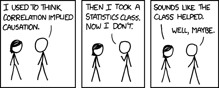
© xkcd

Correlation does not imply causation

• Even if we’ve made sure we’ve done a good job with our sampling, and don’t have biased data, our results are only correlational
• They can tell us what the relationships between variables are, but not what caused them
• There’s a good list in chapter 17 of the The Effect:
  • Someone has a late-night beer, immediately falls asleep, and concludes the next day that beer makes them sleepy
  • You put up a “no solicitors” sign on your door, notice fewer solicitors afterwards, and conclude the sign worked
  • When your dog is hungry, then finds you and whines, and becomes fed and full, then concludes that whining leads to getting fed
  • When a rooster concludes they’re responsible for the sun rising because it rises every morning right after they crow

Correlation is ambiguous causation

• If we have a statistically-significant relationship, something is causing it
• We just don’t know what
• There’s a lot you can do with correlational studies in combination with theory
• Most quantitative planning studies are correlational

Tell me why

• ain’t nothin’ but a heartache
• Sometimes, we really do want to know why
• Theory is a big part of knowing why—how do we think the data generating process works?
• Correlational studies can tell us if the data are at least consistent with theory
• But we still can’t be sure

Why is correlation ambiguous?

• What are the reasons variables \(x\) and \(y\) could be correlated?
• \(x\) causes \(y\)
• \(y\) causes \(x\)
• \(z\) causes \(x\) and \(y\)
• Some combination of the above

The role of regression

• Regression helps us with the third situation
• If there is a variable \(z\), and if we can measure it, controlling for \(z\) in the regression allows us to estimate the relationship between \(x\) and \(y\), separate from the relationship with \(z\)

Front-door and back-door paths

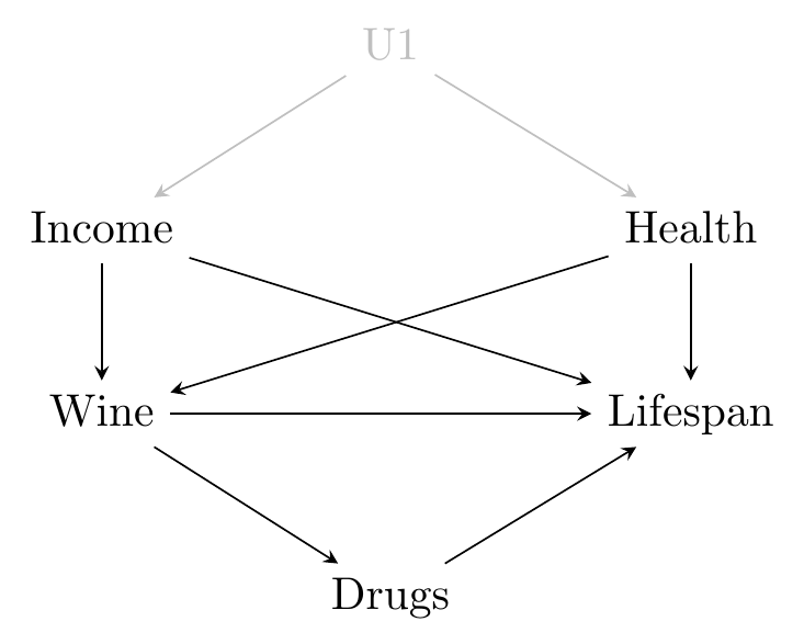
Huntington-Klein (2022)

The ultimate goal

• Control for every other way your variables could be related that is not part of your research question
• Then, your coefficients are the causal effect of the independent variable on the dependent variable
  • Assuming the causality does flow from \(x\) to \(y\) and not \(y\) to \(x\) and your sample is random

What happens if you don’t control for everything?

• Omitted variable bias
• Other coefficients correlated with omitted coefficient are biased
• Remember Simpson’s paradox?

Endogeneity

• Endogeneity is a fancy word for this problem
• Mathematically, it means that the independent variables are correlated with the error term
  • Don’t think too hard about this
• Practically, it means that you have one of the situations above

Terminology of causal inference

• treatment: whatever it is you want to evaluate the causal effect of
• treatment group: the group that receives the treatment
• control group: a group that does not receive the treatment, for comparison purposes
• counterfactual: what would have happened had a treated person instead not been treated, or vice versa

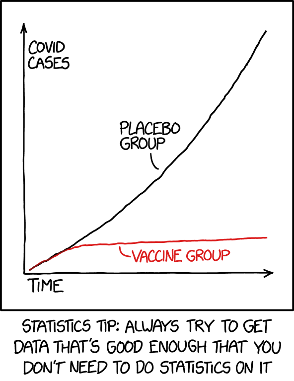
The experimental ideal

• The “gold standard” is the randomized control trial
• You take your sample, and randomly divide people into the treatment group and the control group
• Because you divided the sample randomly, the only difference between the treatment and control group is whether they received the treatment
• Do a hypothesis test, maybe a very simple regression, and you’re done

© xkcd

Randomized control trials in planning

• Randomized control trials are very common in medicine
• They almost never happen in planning
  • In fact, if you ask academic planners about randomized control trials in planning, they will almost all think of the same one: Moving to Opportunity
• We don’t usually get to assign people to residential locations, car ownership levels, etc.
  • And there would be significant ethical concerns with doing so
• Dr. Palm and I are actually working on a randomized control trial for e-bike ownership now—stay tuned!

Moving to Opportunity

• By the 1980s, conditions in inner-city public housing projects were reprehensible, and the projects were highly segregated
• The Section 8 housing voucher program had just been created
• The research question was broadly how deconcentrating poverty would affect those receiving assistance
• Moving to Opportunity assigned volunteer subjects to a treatment group who received housing vouchers restricted to low-poverty neighborhoods, and control groups with unrestricted vouchers or staying in public housing (de Souza Briggs et al. 2010)

Findings from Moving to Opportunity

• Movers reported significantly increased feelings of safety (de Souza Briggs et al. 2010)
• Young children who moved were more likely to attend college, while older children had a mildly negative change (Chetty et al. 2016)
• Movers reported increased mental health (Leventhal and Brooks-Gunn 2003)
• No significant change in work outcomes, on average (Ludwig et al. 2013; de Souza Briggs et al. 2010)

Alternatives to randomized control trials

• We usually don’t get to do randomized control trials
  • As evidenced by the fact that many planners know the randomized control trials in planning by name
• The goal of a randomized control trial is to isolate all other potential sources of a relationship between your dependent variable and treatment
• There are other methods of doing this as well, known as causal inference

Statistical control

• The simplest approach to this is to just control for things that might be confounders
  • e.g. it’s very common to control for demographics
• It requires you to assume that you’ve measured every possible variable that could influence both the treatment and the the dependent variable
• And that there is no endogeneity
• This is usually not very convincing on its own
  • Social science is complicated
  • Knowing things is hard

What to control for

• You want to control for everything you don’t want to measure the effect of
• and nothing you do
• This can depend on your research question
• For instance, suppose you ran a regression of homeownership on race
• Race would probably be significant
• But if you then controlled for income, savings, education, whether your parents owned a home, whether anyone in your family could cosign a loan, etc., race might become insignificant
• Does this mean there is not structural racism in homeownership, or have you controlled for the mechanisms by which structural racism operates?

Fixed effects: controlling for things you can’t (or didn’t) measure

• You don’t always get what you want (to control for)
• Fixed effects let you control for all unobserved attributes of some sampling unit
• For instance, suppose you don’t have a good measure of school quality, but you do know what school everyone in your sample attends

Fixed effects are just dummy variables

• A fixed effect adds a dummy variable for each school; anything that doesn’t vary among students within the same school will then be implicitly controlled for¹
  • When you control for district in the homework, you are adding a fixed effect
• You have to have multiple students from each school for this to work²
• You can’t add any other school-level effects (e.g. average test scores) in your regression if you have school fixed effects

1. most people use a special fixed-effects estimating package, e.g. fixest in R, to avoid proliferation of potentially hundreds or thousands of variables

2. if you didn’t, then the school fixed effect would just perfectly track the dependent variable for the one student in that school

Fixed effects and panel/longitudinal data

• If you have panel/longitudinal data (multiple observations of the same individual), you can have individual-level fixed effects
• This is a separate coefficient for every person in your model, and controls for any attributes of that person that don’t change between observations
• You can’t have other control variables for person characteristics that don’t change over time

Fixed effects

• In some recent research (Bhagat-Conway and Zhang 2023), I found that rush hours are spreading out after the pandemic lockdowns
• We wanted to make sure we weren’t seeing this effect because of a change in what roadway sensors were online before and after the lockdowns
• We included sensor fixed effects (about 3,500) to control for any attributes of where the sensors were
• We could do this because we had many observations from each sensor (and 4.6 million observations overall)

Matching

• In matching, you try to choose observations for your control group that match your treatment group
• Often, this is a 1:1 approach—you use the variables in your data to find the closest match from the control group for each observation in the treatment group
  • But it doesn’t have to be
• Hopefully, by matching on the observed variables, you can create treatment and control groups that only differ because one was treated
• This is somewhat similar to controlling for a lot of things, but with fewer assumptions (e.g. linearity)
• But, like regression, you have to hope that there aren’t things you don’t observe that matter for your outcome

Matching: example

• Kaza and BenDor (2013) looked at the land value impacts of wetland restoration by matching sales near restoration projects with other sales
• They found that immediately adjacent there was a negative effect, but further away the effect was positive

Natural experiments

• A natural experiment is some process in the world that isolates the relationship between the treatment and control, without confounders
• They may come from policy or technology changes, mistakes, natural disasters, etc.

Event studies

• In 2020, new International Maritime Organization rules went into effect restricting the quantity of sulphur allowed in ship fuel
• This reduced sulfur oxides pollution, but also decreased cloudiness over the ocean, potentially exacerbating global warming
• By comparing the before and after periods, Diamond (2023) found a statistically significant increase in warming

Challenges with event studies

• No direct control group; cannot separate effects of things that occurred at the same time
• Diamond (2023) actually used a sophisticated method to create the counterfactual, not a straight before-after comparison

Regression discontinuity

• A regression discontinuity design exploits the fact that some treatments are assigned based on arbitrary cutoffs in some forcing variable (e.g. an income cutoff for a means-tested welfare program, an SAT score cutoff for admission to a prestigious university, first-past-the-post elections)
• While outcomes may vary due to whatever the cutoff is based on, they should vary continuously
• For instance, if you’re measuring post-college earnings, you might expect them to vary based on SAT score
• But if you observed a sharp change right at the cutoff for the prestigious university, that’s probably due to the admission to the prestigious university

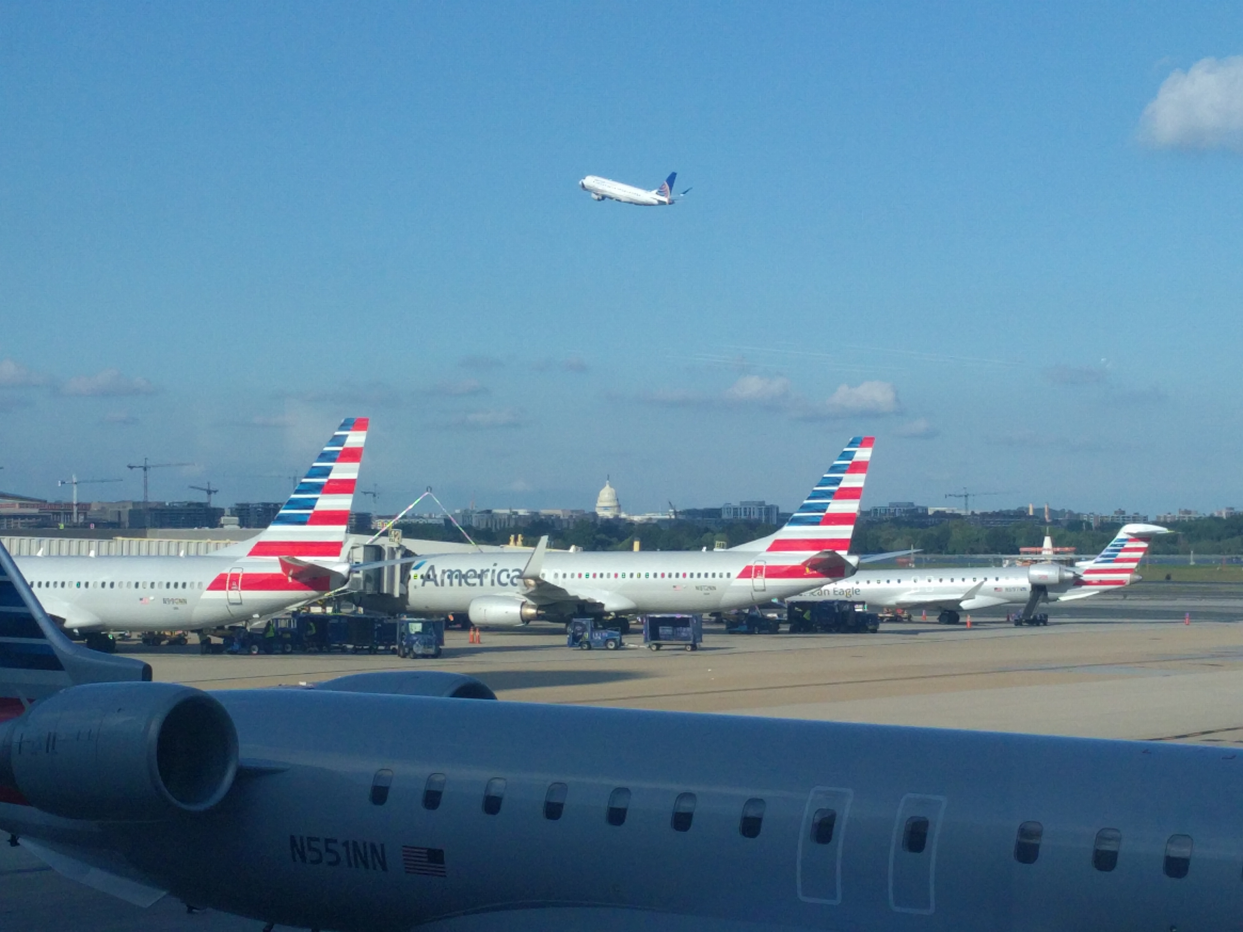
Regression discontinuity, hypothetically

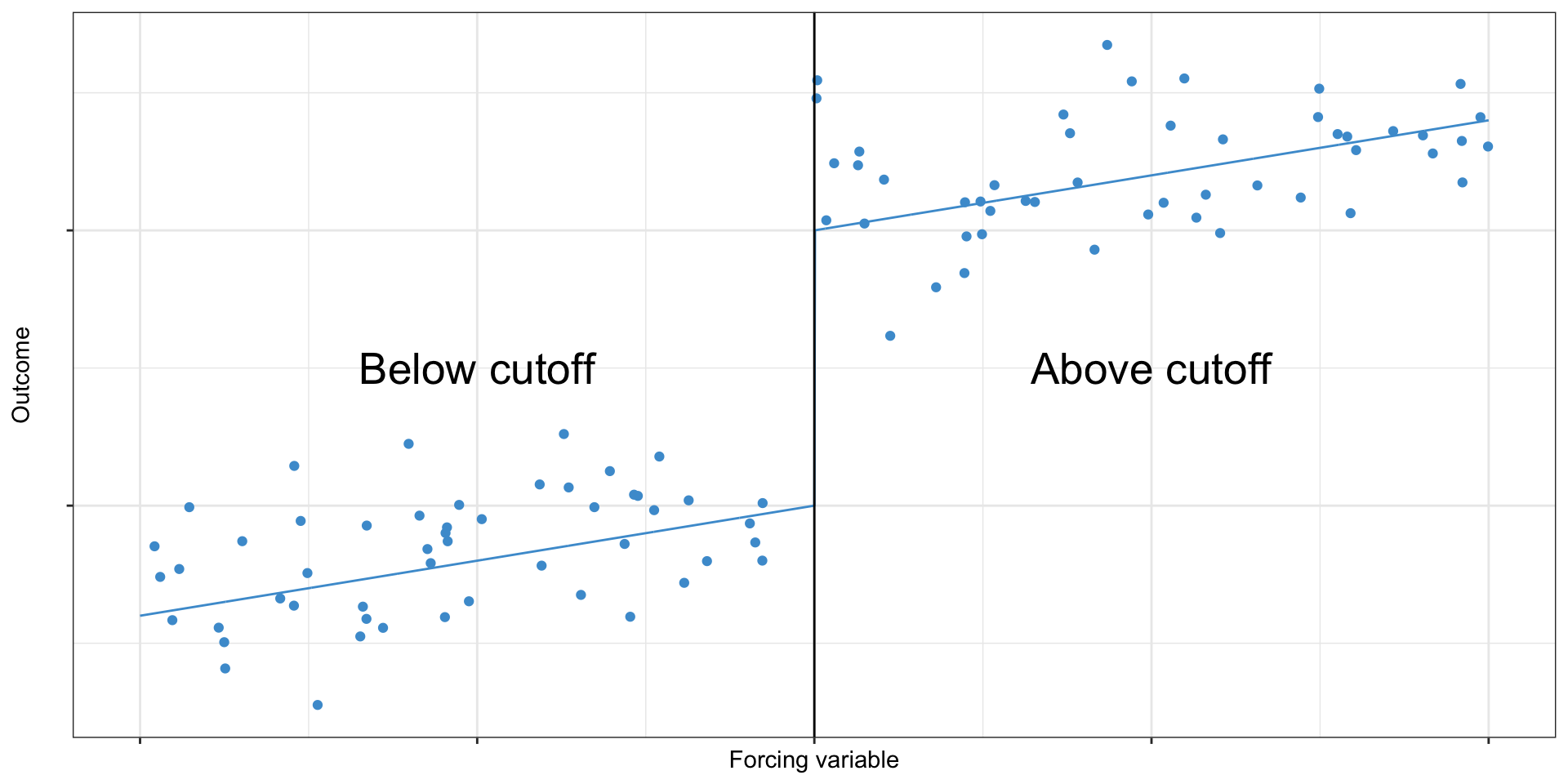
Regression discontinuity

• Airfares are generally more expensive at hub airports dominated by a single carrier (e.g. Atlanta, Charlotte, Newark)
• The AIR-21 act aimed to promote competition at these airports
• It applied to large airports where >50% of traffic is from one or two airlines
• Hubs are probably different from other large airports in all kinds of ways, but airports with 49% vs 51% of service from two carriers are probably pretty similar
• Snider and Williams (2015) uses this to find that the act reduced airfares 13–20% at these airports

Differences in differences

• Event studies can be very useful, but they suffer because many things may change over time
• In differences in differences, you have two groups
  • One treatment group that you observe before and after the treatment
  • One control group that never gets treated
• You assume that, if the treatment group was never treated, it would have the same trend as the control
• You compare the change in the treatment group to the change in the control group

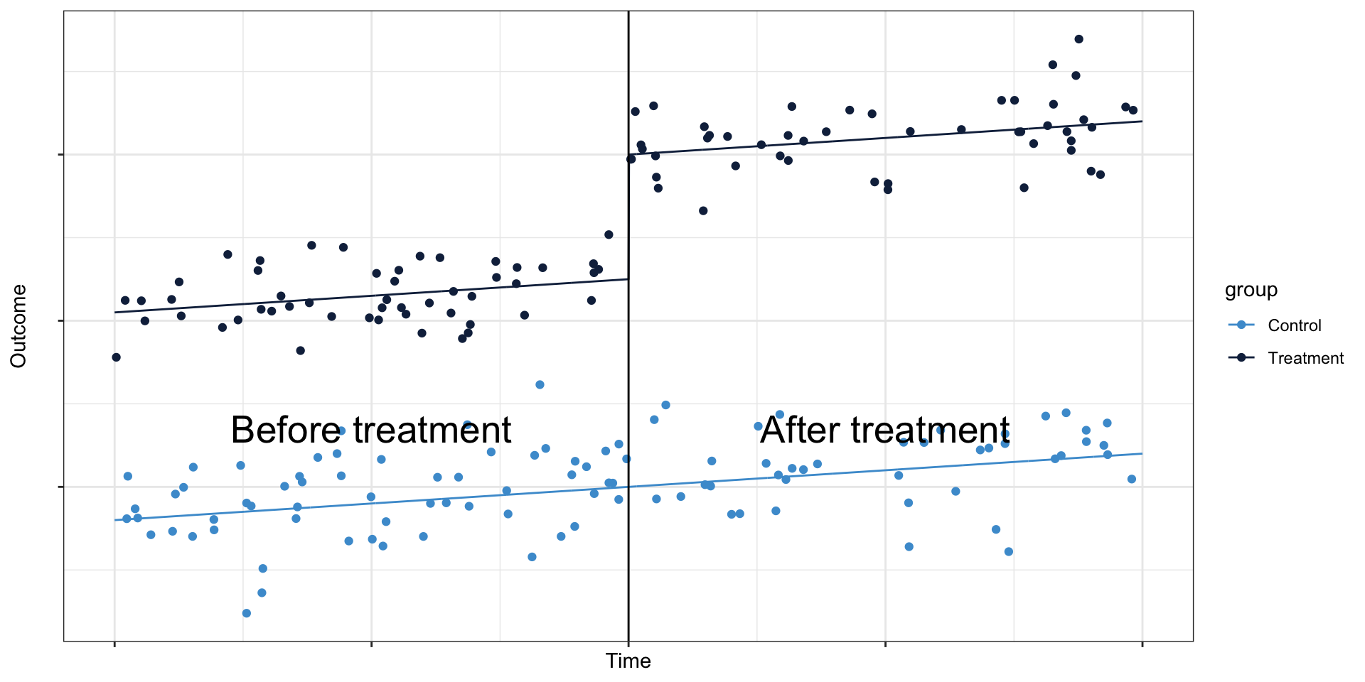
Differences in differences, hypothetically

Pollution is bad

• Air pollution is bad for your health, but it’s hard to test this statistically
• Places with polluted air often have a bunch of other predictors of poor health as well—low access to health care, high poverty, etc.
• In the early 2000s, New Jersey and Pennsylvania replaced tollbooths with E-ZPass electronic tolling lanes, which reduced pollution around tollbooths
• Currie and Walker (2012) found that these changes led to a ~10% reduction in adverse birth outcomes relative to other areas along the same highways

Instrumental variables

• Sometimes we can’t find a clean way isolate the variation in our dependent variable that is specifically caused by our independent variable of interest
• In an instrumental variable approach, we find an instrumental variable (aka instrument) that affects the independent variable of interest, but there is no other conceivable way it could affect the dependent variable
• This can also be used with a randomized control trial with imperfect compliance (e.g. some people assigned to the treatment group didn’t actually get treated, or some people in the control group found a way to get treated)

Instrumental variables

• A very common example is trying to evaluate the benefits of additional schooling
• For instance, maybe we are interested in the effect of staying in high school longer rather than dropping out on wages
• The problem is that the people who drop out of high school earlier are probably different from people who do not
• Most states require students to stay in school until they turn 16
• When they are required to start school varies by state, but there is generally a cutoff date
• People born at different times of year therefore are required to stay in school for more or less time
• Angrist and Krueger (1991) use this to find that the causal effect of another year of high school on wages is about 6%

Sample selection/Heckman models

• A common problem is that your sample is not random because you can’t observe the outcome for some segment of your population
  • And that segmentation is correlated with your outcome
• Classic example is determinants of wages
  • We only observe wages for those who work
  • Whether someone works or not is probably related to how much money they would make if they did
  • Any sample of workers is a non-random sample of the overall population

What the heck, man?

• The Heckman model works with data from a random sample of the population, with missing values for the dependent variable in some subset (e.g. non-workers)
• It is then a two stage model
  • First stage models the probability of being in the subset with non-missing values (e.g. workers)
  • Second stage models the actual outcome
  • Sample selection bias is mitigated by using a function of the results of the first model as a control variable in the second
    • Not just the prediction, but a function of the prediction and error distribution
  • There must be at least one variable that predicts selection but not the dependent variable
• Only corrects for sample selection, not other forms of endogeneity

Sample selection models: example

• Salon et al. (2022) used a sample selection model to estimate the relationships between attitudes, demographics, and telecommute frequency
• Telecommute frequency only observed for those with the option to telecommute
• Preferences for workplace interaction and difficulty getting motivated at home predicted working from home less
• Preferences for working from home predicted working from home more
• Older workers more likely to choose to telecommute every day
• Transit commuters more likely to switch to telecommuting
• Aspects of the home and household—size, extra bedrooms, high-speed internet, presence of children—not predictive of telecommuting

References

Angrist, Joshua D., and Alan B. Krueger. 1991. “Does Compulsory School Attendance Affect Schooling and Earnings?” The Quarterly Journal of Economics 106 (4): 979–1014. https://doi.org/10.2307/2937954.

Bhagat-Conway, Matthew Wigginton, and Sam Zhang. 2023. “Rush Hour-and-a-Half: Traffic Is Spreading Out Post-Lockdown.” PLoS One.

Chetty, Raj, Nathaniel Hendren, and Lawrence F Katz. 2016. “The Effects of Exposure to Better Neighborhoods on Children: New Evidence from the Moving to Opportunity Experiment.” American Economic Review 106 (4): 855–902. https://doi.org/10.1257/aer.20150572.

Currie, Janet, and Reid Walker. 2012. Traffic Congestion and Infant Health: Evidence from E-ZPass. NBER Working Paper No. 15413. National Bureau of Economic Research. https://www.nber.org/system/files/working_papers/w15413/w15413.pdf.

Diamond, Michael S. 2023. “Detection of Large-Scale Cloud Microphysical Changes Within a Major Shipping Corridor After Implementation of the International Maritime Organization 2020 Fuel Sulfur Regulations.” Atmospheric Chemistry and Physics 23 (14): 8259–69. https://doi.org/10.5194/acp-23-8259-2023.

Huntington-Klein, Nick. 2022. The Effect: An Introduction to Research Design and Causality. First edition. A Chapman & Hall Book. CRC Press, Taylor & Francis Group. https://doi.org/10.1201/9781003226055.

Kaza, Nikhil, and Todd K. BenDor. 2013. “The Land Value Impacts of Wetland Restoration.” Journal of Environmental Management 127 (September): 289–99. https://doi.org/10.1016/j.jenvman.2013.04.047.

Leventhal, Tama, and Jeanne Brooks-Gunn. 2003. “Moving to Opportunity: An Experimental Study of Neighborhood Effects on Mental Health.” American Journal of Public Health 93 (9): 1576–82. https://doi.org/10.2105/AJPH.93.9.1576.

Ludwig, Jens, Greg J. Duncan, Lisa A. Gennetian, et al. 2013. “Long-Term Neighborhood Effects on Low-Income Families: Evidence from Moving to Opportunity.” American Economic Review 103 (3): 226–31. https://doi.org/10.1257/aer.103.3.226.

Salon, Deborah, Laura Mirtich, Matthew Wigginton Bhagat-Conway, et al. 2022. “The COVID-19 Pandemic and the Future of Telecommuting in the United States.” Transportation Research Part D: Transport and Environment 112 (November): 103473. https://doi.org/10.1016/j.trd.2022.103473.

Snider, Connan, and Jonathan W. Williams. 2015. “Barriers to Entry in the Airline Industry: A Multidimensional Regression-Discontinuity Analysis of AIR-21.” The Review of Economics and Statistics 97 (5): 1002–22. https://doi.org/10.1162/REST_a_00455.

Souza Briggs, Xavier de, Susan J Popkin, and John Goering. 2010. Moving to Opportunity: The Story of an American Experiment to Fight Poverty. Oxford University Press.

This work by Matthew Bhagat-Conway is licensed under a Creative Commons Attribution 4.0 International License.